Saturday Evening Post Archives: Engineering a Smart Search Solution

This is a deeply technical article, complete with code snippets, machine learning, algorithms, and all that jazz. We’ll get to that in a minute, but first, let’s start with a bit of a “lyrical” introduction.

It all started with Norman Rockwell. I’m generally into painting and try to dabble a bit myself, but in my tastes, I am very conservative—even old school, you might say. Shortly before that day, a friend and I were reminiscing about famous American illustrators, and I became engrossed in a collection of Rockwell illustrations in The Saturday Evening Post. They were extraordinarily vivid and dynamic, and they exuded that good old America.

Viewing his illustrations online offers one experience; holding a magazine that features them is quite another. Beyond its cover, the magazine boasts over a hundred pages filled with an array of content, including fiction, news and current events, humor and satire, as well as editorials, opinion pieces, and reflective articles on history and nostalgia.

So I decided to find a collection of magazines and browse through them myself. Well, if this magazine was read by all of America, it must be in every major library, right? After several attempts, I realized that there was only one option: to find it in the Library of Congress.

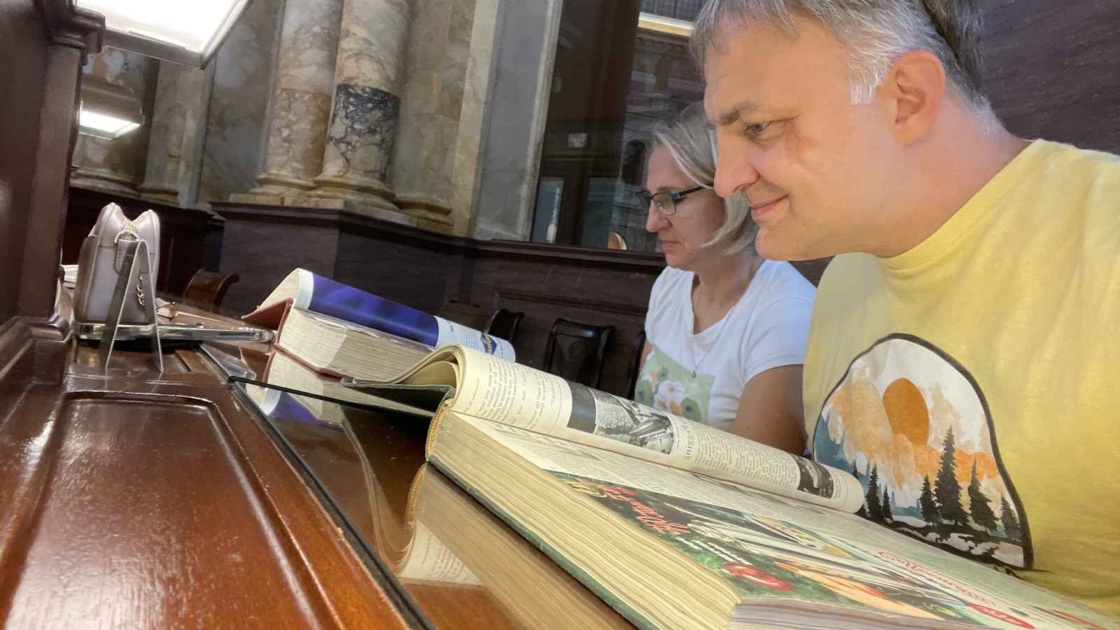
Registering at the Library of Congress is relatively quick and straightforward, but obtaining the magazine archives took two days. On the first day, by the time I had registered, toured all the halls, and figured out where and how to search, it was already lunchtime. Then, after submitting my request and waiting for an hour and a half as they searched, they told me they hadn’t found anything, and by then, everything was closing. The next time, I arrived earlier, and although the search took a long time again, we finally received the long-awaited archives.

I specifically chose issues from May 1945 to see how much space the war theme occupied in the press at the time. The year 1950 was chosen more or less at random.

Upon returning, I unexpectedly discovered that the archives of The Saturday Evening Post are available on its official website. Where had I been before! They aren’t free, but the fee is affordable, and I immediately subscribed to the magazine itself. The subscription included access to the archive.

The Saturday Evening Post was first published in 1821, two hundred years ago. It is one of the oldest magazines in the United States. Historically, it was a weekly publication and played a significant role in American culture. The magazine featured a mix of fiction, non-fiction, and features that appealed to a broad readership. With access to the archive, you could pick any issue from it, but there was no search box.

There was no search through either the entire archive or a selected issue because all the pages were images.

It looked like a challenge!

What if we recognize all the pages, convert them to text, and then continue searching through this text using vector search? How would it work with such volumes? Can it be combined with traditional keyword search?

I quickly made a prototype that worked with one issue of the magazine. The magazine had over a hundred pages, so there was plenty of content for experiments. You could choose any issue, or several, or a dozen. It took all weekend to develop the prototype.

The processing pipeline involved four phases:

I created a prototype, and now I needed a big corpus to play with.

Contacting Saturday Evening Post

As I mentioned above, I had subscribed to the digital edition of The Saturday Evening Post, hoping to access its archives not only via the browser version but also via its iOS app. When I encountered registration issues, I suspected a bug and contacted customer support. Surprisingly, the person who responded was the Technology Director of The Saturday Evening Post, Steve Harman. He explained that the archives were designed to be accessed only through a desktop.

And then I thought, why not suggest making a search module, since we were already in touch?

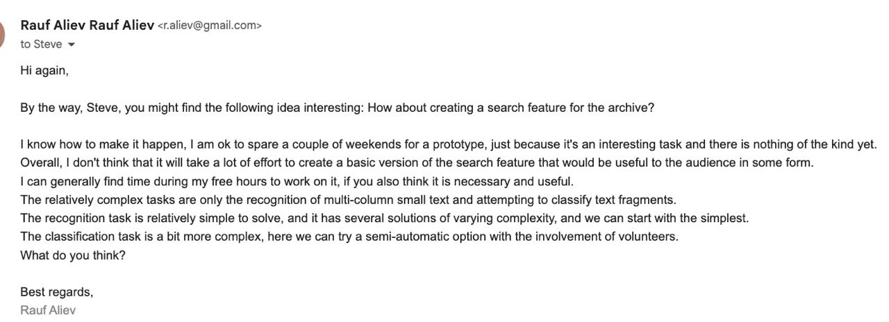
This letter initiated an active exchange of emails and calls. Over several weekends, I experimented with various methods of indexing, text cleaning, and classification. Eventually, I moved to the next level and indexed the magazine’s archive spanning 120 years.

Steve shared that all pages had already been recognized, but the effort required to extract them from their system exceeded the complexity of recognition within my capabilities. Moreover, the overall recognition quality on my end turned out to be quite sufficient for prototype development.

Extracting Magazine Page Images

There were various sources of images available at different phases of the project.

When I worked with PDF files, I extracted images using ImageMagick’s convert:

convert -density 300 input.pdf -quality 100 page-%03d.png

When I had access to the server, I downloaded them with a script supporting parallel streams:

def download_file(url, folder):
    response = requests.get(url)
    if response.status_code == 200:
        filename = os.path.join(folder, os.path.basename(url))
        with open(filename, 'wb') as file:
            file.write(response.content)
        print(f"File downloaded to {filename}")
    else:
        print(f"Failed to download file from {url}")

def download_parallel(num1, num2_list, folder):
    with concurrent.futures.ThreadPoolExecutor(max_workers=5) as executor:  # You can adjust the number of workers
        futures = []
        for num2 in num2_list:
            url = get_download_url(num2);]
            futures.append(executor.submit(download_file, url, folder))

        for future in concurrent.futures.as_completed(futures):
            try:
                future.result()
            except Exception as e:
                print(f"Download failed with error: {e}") 

Text Extraction

The JPGs were converted into text with Tesseract OCR:

tesseract page-1.png out --psm 1 -l eng

The --psm 1 option in the Tesseract command-line tool stands for “Page Segmentation Mode 1.” In Tesseract, Page Segmentation Modes (PSMs) dictate how the OCR (Optical Character Recognition) engine should interpret the layout of the page it’s processing. This means that Tesseract will try to detect any orientation or script directions automatically and then segment the page to interpret different text areas accordingly. Specifically, for this page:

The extracted text will look like this:

As you can see, “Let me take…” and “track down stocks” are separated. This problem cannot be addressed with psm=1, but without it, the system would join the fragments from the left and right columns line by line, which would make it impossible to extract meaningful sentences.

By using the multiprocessing module, the script can process multiple images in parallel. This takes advantage of multi-core processors to significantly reduce the total processing time compared to processing images sequentially, which is what happens in a typical command-line execution:

import os
import glob
import multiprocessing
from PIL import Image
import pytesseract
import sys

def process_image(image_path):
    try:
        img = Image.open(image_path)
        text = pytesseract.image_to_string(img, config='--psm 1')
        output_path = os.path.splitext(image_path)[0] + '_raw.txt'
        with open(output_path, 'w', encoding='utf-8') as output_file:
            output_file.write(text)
                print(f'Processed: {image_path}')
    except Exception as e:
        print(f'Error: {image_path}: {str(e)}')


if __name__ == '__main__':
    input_folder = sys.argv[1]
    image_files = glob.glob(os.path.join(input_folder, '*.jpg'))
    pool = multiprocessing.Pool()    
    pool.map(process_image, image_files)
    pool.close()
    pool.join()

This is how it worked with the scans:

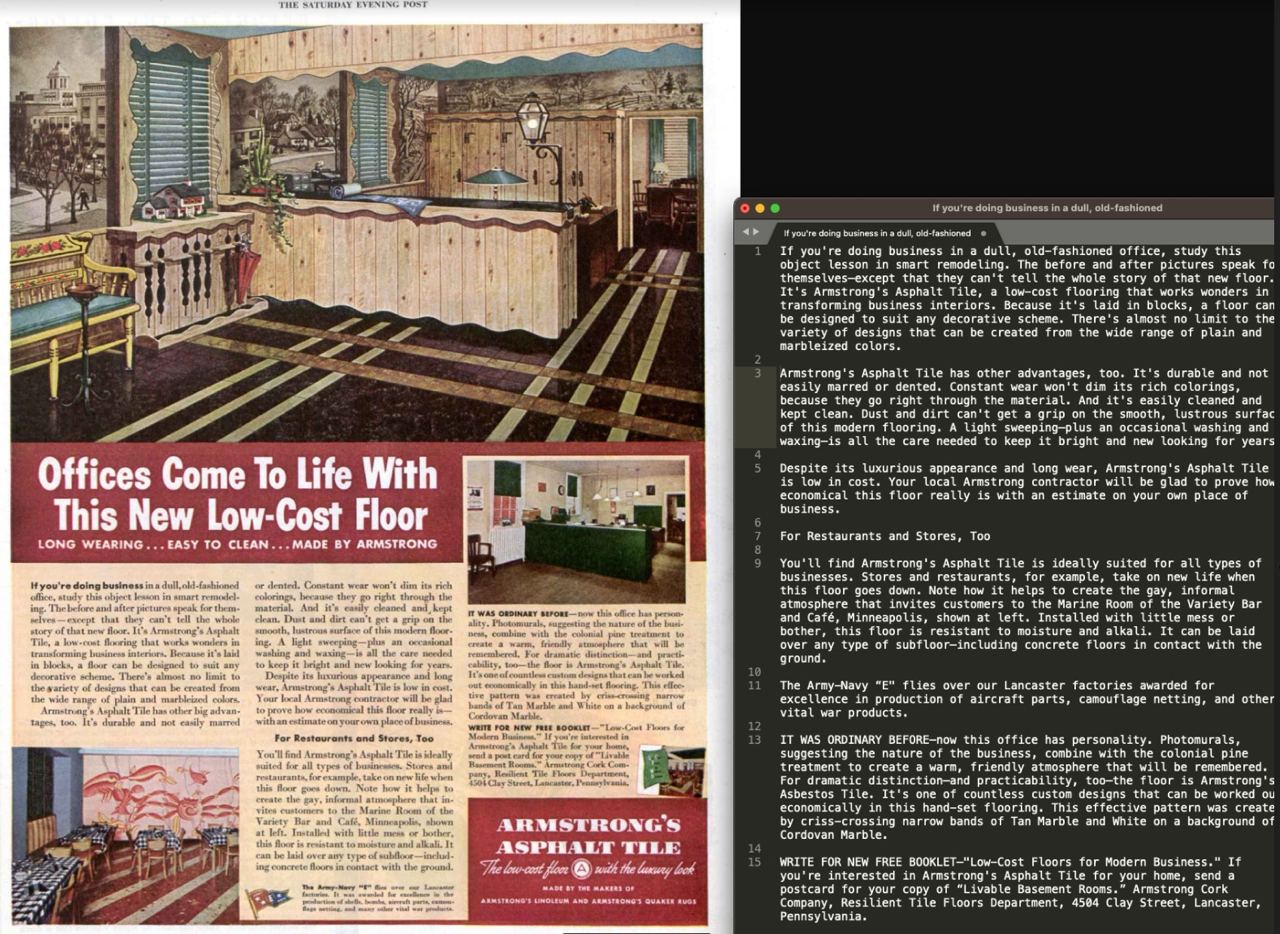
OCR may not accurately recognize distorted, curved, or slanted text on the pages. Using OpenAI for this purpose could probably also be a good option.

Anyway, recognition needs to be done only once. The archive is not small, but it is finite.

Performance-wise, on my MacBook i7, recognition took around two seconds per image.

Text Cleanup

The next phase is text cleanup. It was required because the OCR process was not perfect (as the source images were not perfect either), and some words were broken or skewed. I tried various ways to fix such errors, and one approach turned out to be great: the OpenAI Completions API. My script sent raw OCR output to OpenAI with the following prompt: “Don’t change text. Just fix the formatting.” Together with the formatting, it fixed broken words and typos. Version 3.5 was not quite accurate. It worked in about 90% of cases, but sometimes it hallucinated and added something out of thin air (look at the second half of the text):

GPT-4 was much more accurate. I saw some hallucinations too, but all of them were minor.

The main challenge with recognition was that it was difficult to distinguish between, say, advertisements and the main text on the magazine pages. Some pages have two articles on them. The OCR software blended everything together. I am writing about classification as an attempt to perform this separation.

For vector search, it was necessary to split the text into sentences. To do this, sentences needed to be composed of words, sometimes separated by a hyphen. Overall, OpenAI handles this quite well, but it’s often not feasible to use it because it’s not free. The simplest way to split text into sentences involves regular concatenation of words that have a hyphen at the end of a line with the first word of the next line, as well as using an NLP library for sentence segmentation:

import os
import glob
import multiprocessing
import spacy
import re
import sys
nlp = spacy.load("en_core_web_sm")

def process_text(text_path):
    try:
        with open(text_path, "r", encoding="utf-8") as input_file:
            text = input_file.read();
        
            text = text.replace('\n', ' ')
            text = text.replace('- ', '')
            text = text.replace('-', ' - ')

            doc = nlp(text)
            res = "";

            for idx, sentence in enumerate(doc.sents, start=1):
                cleaned_tokens = []
                for token in sentence:
                    if token.text == '-' and cleaned_tokens:
                        cleaned_tokens[-1] += '-'
                    else:
                        cleaned_tokens.append(token.text)
                
                cleaned_sentence = ' '.join(cleaned_tokens)
                cleaned_sentence = re.sub(r'\s+', ' ', cleaned_sentence).strip()  
                res = res + cleaned_sentence + "\n";

            output_path = os.path.splitext(text_path)[0] + '_sentences.txt'
            
            with open(output_path, 'w', encoding='utf-8') as output_file:
                output_file.write(res)
            
            print(f'Processed : {text_path}')
    except Exception as e:
        print(f'Error:  {text_path}: {str(e)}')

if __name__ == '__main__':
    input_folder = sys.argv[1]+"/";
    
    text_files = glob.glob(os.path.join(input_folder, '*_raw.txt'))
    
    pool = multiprocessing.Pool()
    pool.map(process_text, text_files)
    pool.close()
    pool.join()

Extracting Entities from the Text

I also experimented with extracting entities from the text—such as cities, countries, names, and brands. While it worked well for small datasets, it produced questionable results for the whole archive. But for completeness, I’ll show how they were extracted:

def extract_entities(text):
    doc = nlp(text)
    entities = {}
    
    entities_cnt = Counter()
    for ent in doc.ents:
        entity_type = ent.label_
        entity_value = ent.text.lower()

        if entity_type not in entities:
            entities[entity_type] = {}
        
        if entity_value not in entities[entity_type]:
            entities[entity_type][entity_value] = {"value": entity_value, "count": 0}
        
        entities[entity_type][entity_value]["count"] += 1

    return entities

def process_text(text_path):
    try:
        output_path = os.path.splitext(text_path)[0] + '_entities.json'
        with open(text_path, "r", encoding="utf-8") as input_file:
            text = input_file.read()
            
            entities = extract_entities(text)
            
            output_path = os.path.splitext(text_path)[0] + '_entities.json'
            
            flat_entities = [{"entity_type": entity_type, "value": list(entity_dict.values())} for entity_type, entity_dict in entities.items()]
            
            with open(output_path, 'w', encoding='utf-8') as output_file:
                json.dump(flat_entities, output_file, ensure_ascii=False, indent=4)  
           
            
            print(f'Processed: {text_path}')
    except Exception as e:
        print(f'Error {text_path}: {str(e)}'

For example, for the following text (1933, November 18, page 1):

“THE SATURDAY EVENING POST An Illustrated Weekly Founded A ? Di 1728 éy Benj . Franklin 10c . in Canada NOVEMBER 18 , 1933 5cts . THE COPY 85 Ea SD aS SA ATS SSS a MEN AGAINST THE SEA — By HALL AND NORDHOFF”

the system extracted:

PERSON : “benj”,
ORG: “franklin”, “ea sd”,
GPE: “canada”

In other words, a straightforward approach to classifying words from the OCR output doesn’t work well.

However, I found some use for the entities extracted from the thousands of pages. I had a script that created a map of the most frequent topics, names, and brands. It helped to see what was being discussed in different decades.

Search Results

I experimented with highlighting the search keywords directly on the pages, but later found this approach inconvenient. With fuzzy search, the documents may not contain any of the keywords, but at the same time, they may be relevant to a query.

This is what I had using the query “Armstrong Asphalt Tile.”

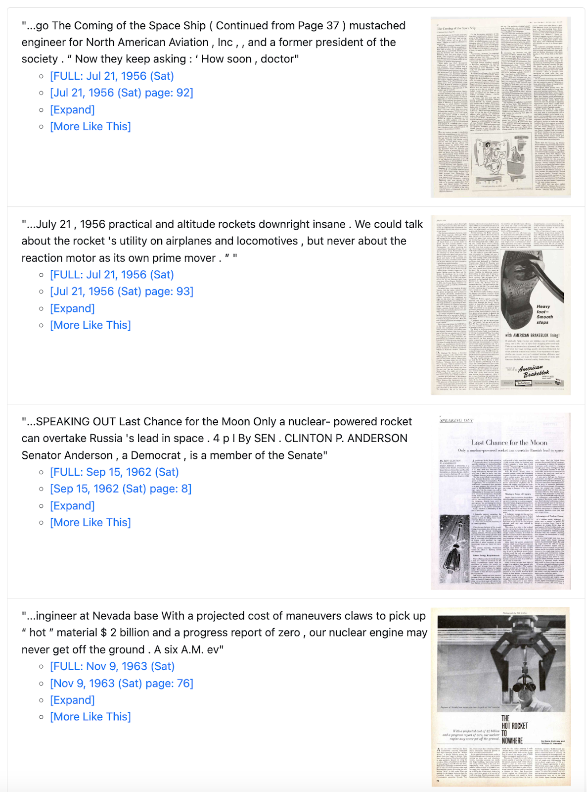
This is how an item in the search results looked (the query was “rocket, space”):

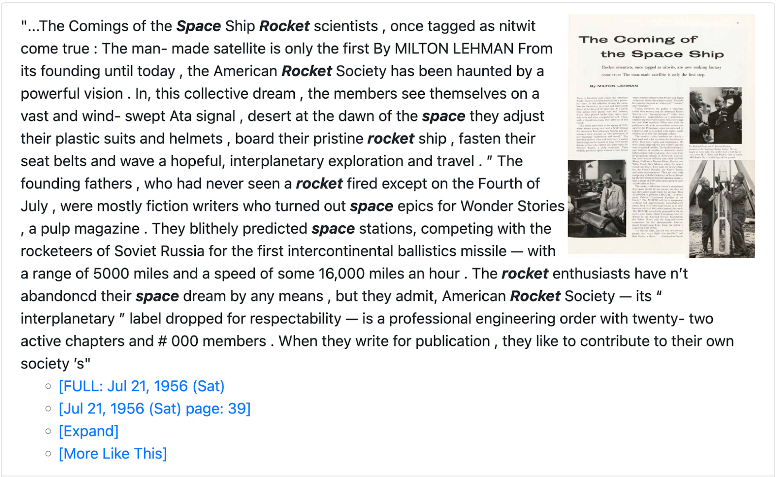
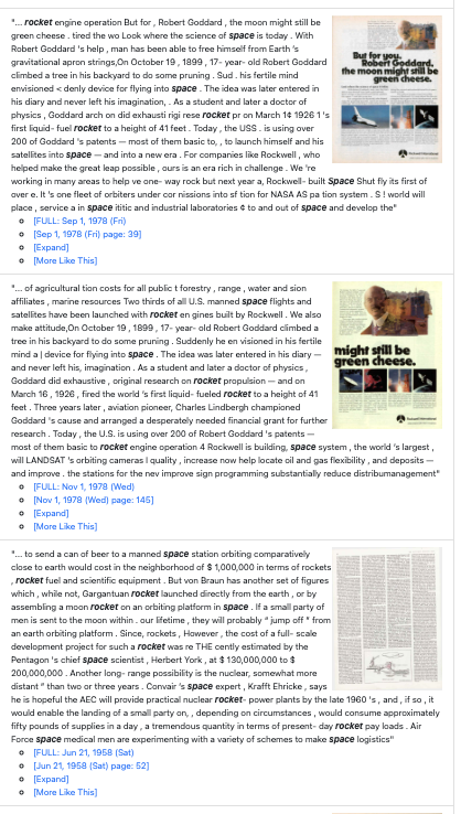
“More like this” shows pages similar to the selected one (actually one from above). We see that the continuation of the same article is here, as well as similar-topic articles from other years.

This is how a list of items looks:

Search Engine

I considered two search engines:

• Experimental — Vector Search.
• Conventional — Apache Solr-based.

Vector Search

Actually, the entire experiment was conceived because of vector search. It was interesting to index large volumes and see how fuzzy search would work. Let’s start with what it eventually produced.

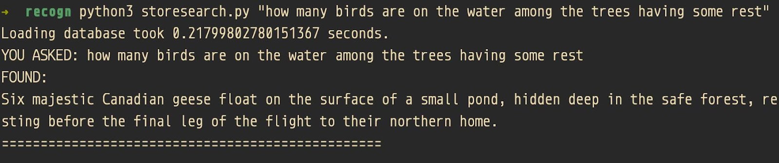
In the example below, I searched for magazine pages using the following query:

“How many birds are on the water among the trees having some rest”

The query is far from natural. It was made up to test the search engine.

Look at what the search engine returned:

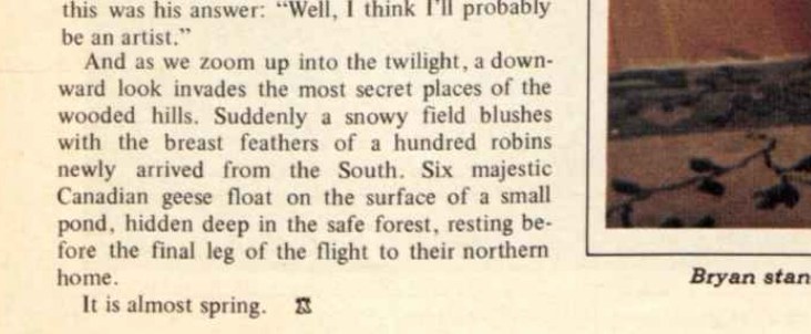
“Six majestic Canadian geese float on the surface of a small pond, hidden deep in the safe forest, resting before the final leg of the flight to their northern home”

As you can see, there are almost no words from the original query, but the meaning is the same. This search by meaning is what makes vector search so interesting.

Another example:

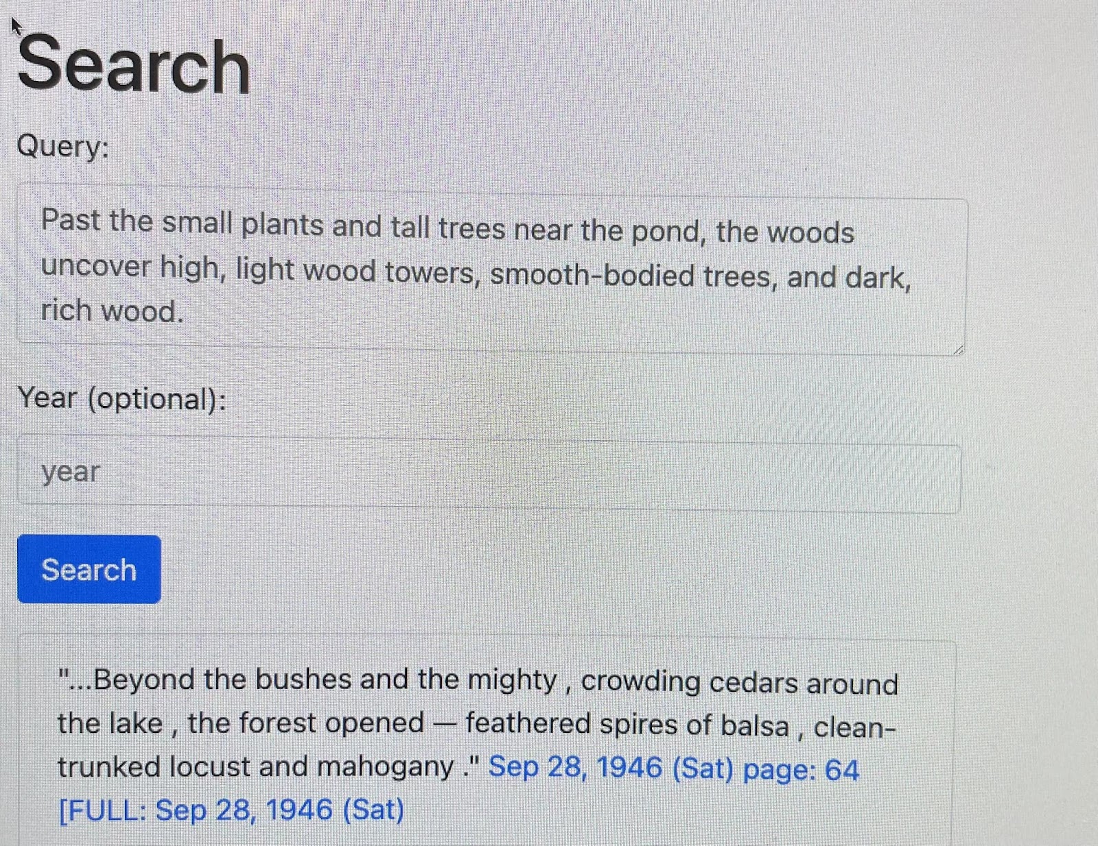
The vector search uses the following technologies:

• LangChain as an interface for OpenAI embeddings
• OpenAI Embeddings API
• FAISS as a vector store

Choosing FAISS for vector storage probably wasn’t the best idea. When I first started working on this topic, there were only a few well-documented solutions available, but things have changed now. Specifically, at that time with FAISS, it was difficult (or impossible) to perform filtering along with searching for documents similar to the query—what is called hybrid search, where sparse vectors meet dense vectors. Solr 9 now generally allows implementing such a search.

See a very convenient table for this purpose: https://superlinked.com/vector-db-comparison/

index ='faiss_index_openai';
…
loader = DataFrameLoader(df, page_content_column='page_content')
documents = loader.load()
text_splitter = RecursiveCharacterTextSplitter(chunk_size=1000, chunk_overlap=0)
texts = text_splitter.split_documents(documents)
embeddings = OpenAIEmbeddings(openai_api_key="...")
db=FAISS.from_documents(texts, embeddings)
if os.path.exists(index):
    local_index=FAISS.load_local(index, embeddings)
    local_index.merge_from(db)
    local_index.save_local(index)
else:
    db.save_local(index)
print(db.similarity_search_with_score('Norman Rockwell'))

Using OpenAIEmbeddings is generally a good idea, but you pay for each call. However, it is affordable:

• text-embedding-3-small: 62,500 texts per dollar, 1,536 dimensions
• text-embedding-3-large: 9,615 texts per dollar, 3,072 dimensions
• text-embedding-ada-002: 12,500 texts per dollar, 1,536 dimensions

In the code above, I used the default model for OpenAIEmbeddings(), which was text-embedding-ada-002.

In fact, it was not a good choice for this purpose because ADA’s dimensions cannot be reduced, unlike the small model (to 256, for example), which is also faster and less expensive.

So if I built the same solution again, I would consider not using FAISS and text-embedding-ada.

Without OpenAI?

I also developed an alternative solution where embeddings were built locally without any help from the OpenAI API.

FAISS_INDEX_PATH="faiss_index"
loader = ReadTheDocsLoader("texts/")
text_splitter = RecursiveCharacterTextSplitter(
    chunk_size = 300,
    chunk_overlap  = 20,
    length_function = len,
)
docs = loader.load()
chunks = text_splitter.create_documents(
    [doc.page_content for doc in docs], 
    metadatas=[doc.metadata for doc in docs])
model_name = "sentence-transformers/all-mpnet-base-v2"
model_kwargs = {'device': 'cpu'}
embeddings = HuggingFaceEmbeddings(model_name=model_name, model_kwargs=model_kwargs)
db = FAISS.from_documents(chunks, embeddings)
db.save_local(FAISS_INDEX_PATH)

Performance-wise, it took 11 minutes to index 700 KB of text (about 7,000 sentences and thus embeddings) with the local embedding all-mpnet-base-v2 (738 dimensions), which is most likely much worse than OpenAI’s. Additionally, indexing slows down as the number of vectors in the database grows. After some point, I dropped this solution because even overnight runs were not making good progress.

149,979 sentences from 35 journals over two years (1966 and 1989) were indexed (only indexed, without recognition) in 9 minutes and 6 seconds.

The problem with vector search is that the index size grows fast, and each new merge into the index takes longer with every new document. The size of the FAISS database containing all sentences from journals over five years was 6 gigabytes. Calculations show that the size of the database for 100 years would be 120 gigabytes, but the problem is that the indexing time also increases, and I probably would never have waited for indexing on my laptop. But even if the problem were only with indexing, to use this FAISS index, you need to load the database into memory. And I don’t have, and won’t have, 120 gigabytes of memory. That’s why I abandoned this idea. However, the approach generally works for volumes smaller than the available RAM.

Since we started with Rockwell, here is one of the first examples:

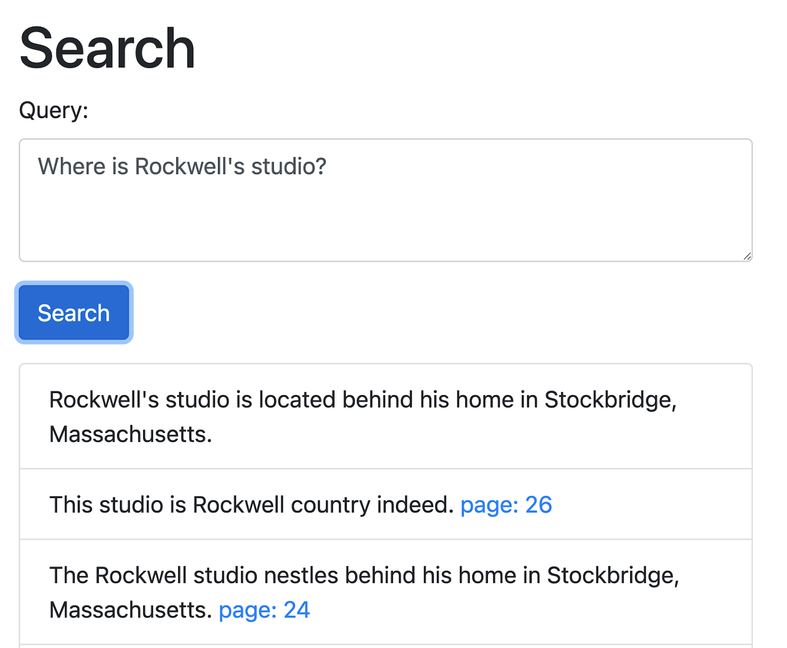
Solr Search

Alongside FAISS, LangChain, and OpenAI embeddings, I also built a conventional Solr index. Overall, Solr 9 also supports vector search (Dense Vector Search), and I, of course, tested it as well, but the issue of how to create vectors for sentences within the existing budget and hardware remains the same. After all, this project is non-commercial. Therefore, Solr is used here for its traditional purpose: reverse-index search by keywords.

However, the Solr “traditional” search configuration was accompanied by “non-traditional” query preprocessing and, on top of that, a reranking algorithm.

Let’s start with the query preprocessing. For the query

Query:

Norman Rockwell

the script sends the following to Solr:

SCORE CALC COMPONENTS:
page_content_text:"Norman Rockwell"^30
page_content_text:"Rockwell"^10
page_content_text:"Norman"^10

and for the query

a classic New England home

Solr receives the following:

SCORE CALC COMPONENTS:
page_content_text:"a classic New"^100
page_content_text:"a classic"^30
page_content_text:"England home"^30
page_content_text:"New England"^30
page_content_text:"New England home"^100
page_content_text:"England"^10
page_content_text:"classic"^10
page_content_text:"classic New"^30
page_content_text:"classic New England home"^150
page_content_text:"a classic New England"^150
page_content_text:"classic New England"^100

I explained this algorithm in my article a few years ago, “Enhanced multi-word synonyms and phrase search”. Notice that the longer the phrase match, the more it contributes to the final score. There are still some imperfections: the articles should be treated differently if they are at the beginning of the subphrase. But even with that, it works fine.

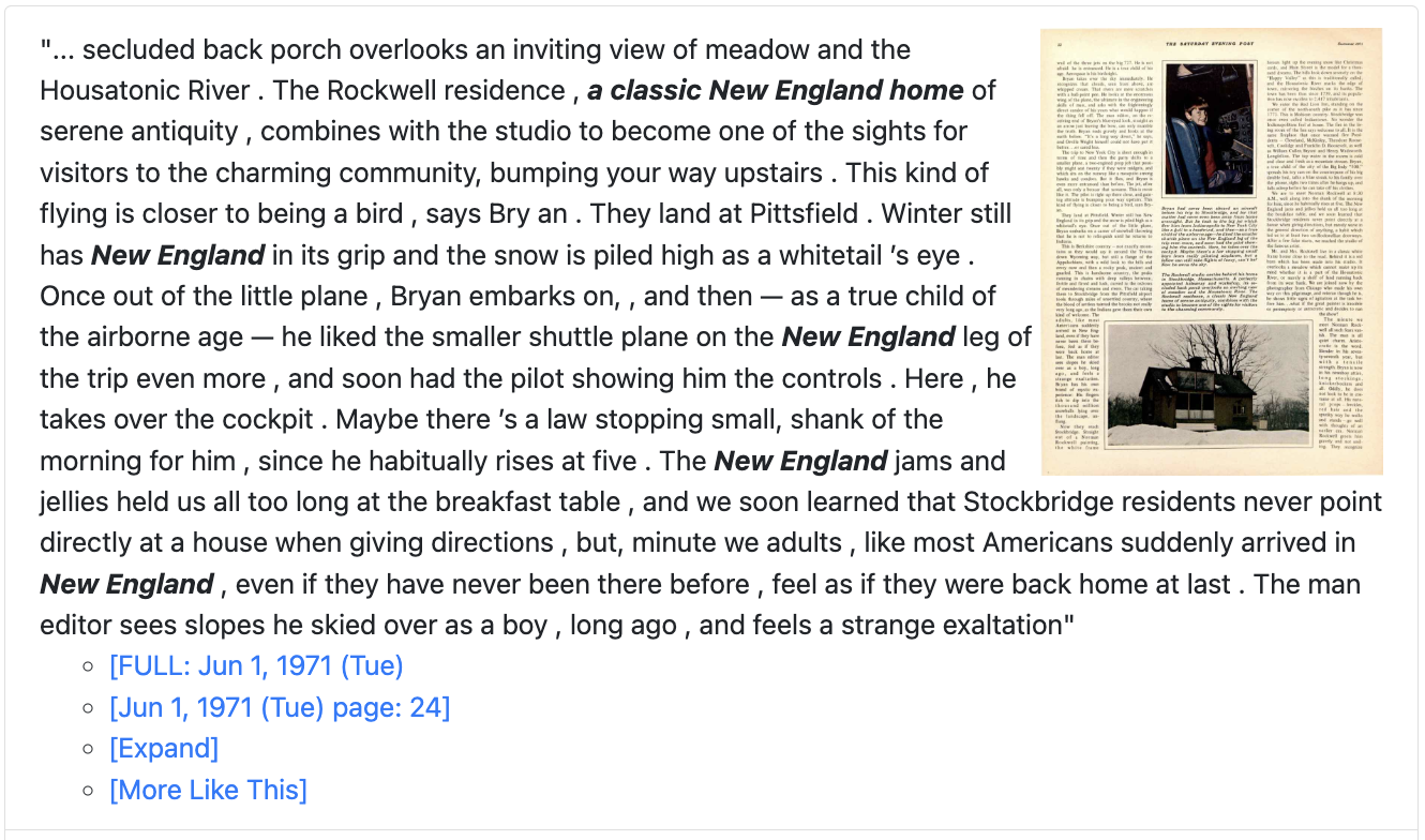
Let’s see what happens if we send a phrase query.

Query

"New England home"

is converted to

SCORE CALC COMPONENTS:
page_content_text:"New England home"^100

Compare that with

Query

New England home

(without quotes)

is converted to

SCORE CALC COMPONENTS:
page_content_text:"New England"^30
page_content_text:"New England home"^100
page_content_text:"England"^10
page_content_text:"England home"^30

What if we mix a phrase and non-phrase?

Query sent to the app:

"New England home" Little Gargle

Query sent to Solr:

SCORE CALC COMPONENTS:
s
page_content_text:"Little Gargle"^30
page_content_text:"New England home Little"^150
page_content_text:"Gargle"^10
page_content_text:"New England home"^100

Notice that the phrase “New England home” doesn’t break in the middle. And consecutive terms are considered as a possible phrase.

There are some special characters. “Minus” means excluding:

-"New England home" Gargle

excludes the whole phrase “New England home”:

Query:

SCORE CALC COMPONENTS:
page_content_text:"Gargle"^10

FILTERS:
-page_content_text:"New England home"

Additionally, the system supports a tilde prefix operator, which is designed to work with word forms:

For example

~germs

is converted into

Query:

SCORE CALC COMPONENTS:
page_content_text:"germ"^10
page_content_text:"germs"^10

and it also supports phrases:

~"these germs"

is converted into

SCORE CALC COMPONENTS:
page_content_text:"these germs"^10
page_content_text:"these germs"^30
page_content_text:"theses germ"^10
page_content_text:"theses germ"^10

if more than one term uses a tilde operator, for example,

~these ~germs

the query for Solr will be converted into

SCORE CALC COMPONENTS:
page_content_text:"these germ"^30
page_content_text:"these germs"^30
page_content_text:"germ"^10
page_content_text:"germs"^10
page_content_text:"theses"^10
page_content_text:"theses germ"^30
page_content_text:"theses germs"^30

Of course, for English, word forms are not as important as they are for French, Russian, Italian, or German.

Additionally, the search query can have some special components:

YEAR:xxxx boosts the results closer to the specified year.

LIKETHIS:id returns results similar to the item with ID=id.

PERSON:, ORG:, GPE: are used for boosting the entity match (see entity recognition above).

Facets

In my PoC, there is only one facet: year.

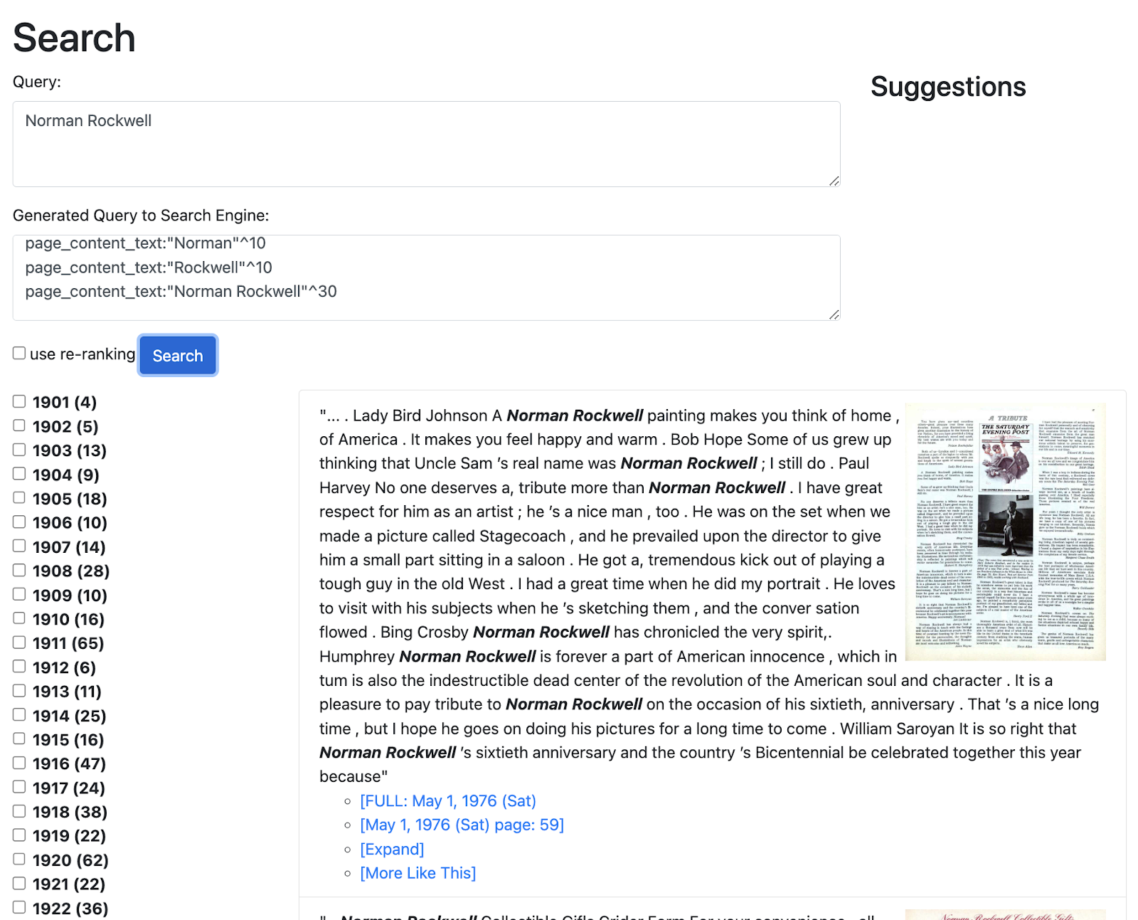
Reranking

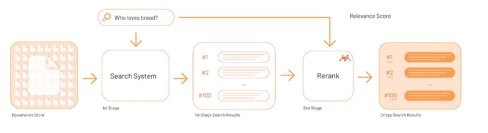
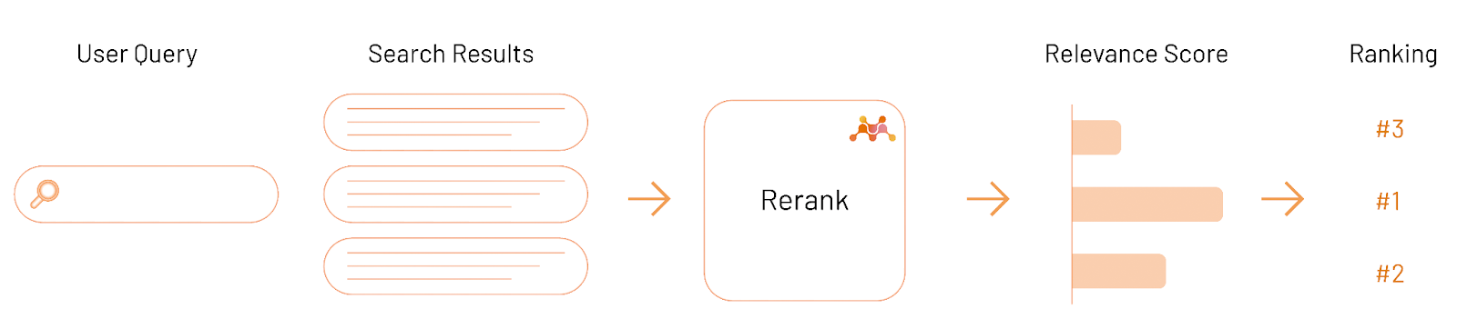
Reranking is applied after a first-stage retrieval step, which returns the first N documents (in my case, N=100). The reranking model from mixedbread.ai is applied at the second stage to get the most relevant candidates to the top. The decision of which of them are more relevant to a query is up to the model.

(The diagrams below are from mixedbread.ai.)

The code for reranking:

from sentence_transformers import CrossEncoder
model = CrossEncoder("mixedbread-ai/mxbai-rerank-base-v1")

def rerank(query, docs):
    if (model):
        documents = [doc["page_content_text"] for doc in docs]
        ranked_results = model.rank(query, documents, return_documents=False, top_k=len(docs))
        sorted_docs = [docs[result['corpus_id']] for result in ranked_results]    
        return sorted_docs

…
response["response"]["docs"] = rerank(query, response["response"]["docs"]); 

For more information about this reranking model, see the blog post.