
Why I needed this
I keep running into the same situation. I need a diagram that exists only as an image: a screenshot of an architecture diagram from someone else's slide deck, a PNG from old documentation, an export from a PDF whose source file was lost along with its author. All it needs is one arrow and two labels fixed, but I end up redrawing the whole thing.
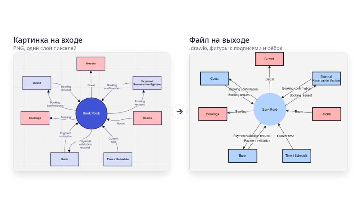
I wanted a tool that takes a raster image and gives back, say, a .drawio file where every rectangle is a rectangle, every label is text, and every arrow is an edge between two nodes. From there, you edit whatever you need.
Here's how I got there, from assembling rectangles out of individual line segments to pairing computer vision with a multimodal model, along with a breakdown of what breaks along the way. Every image in this article is the output of a run on my machine with no manual touch-ups, so you'll see plenty of errors in them. The code is on GitHub; the link is at the end. Feel free to use it.
This solution relies heavily on both AI and computer vision. Let's start with vision, since the input is, after all, an image.
A tracer solves a different problem
The first thing that comes to mind is a tracer: potrace, Image Trace in Illustrator, any "raster to vector" tool. These tools produce outlines and Bézier curves. The image stops pixelating when you zoom in, but it doesn't become an editable diagram. A rectangle turns into a closed curve, artifacts included; text turns into a set of letter silhouettes; an arrow turns into a filled shape. You can't move a node and have the arrow follow, because there is neither a node nor an arrow in the file.
What's needed here is an object model: a list of nodes with coordinates, size, shape, label, and style, plus a list of edges with direction and labels. That's reverse engineering: recovering the document from the final render it produced.
What are we recovering? Node boundaries and shapes, which in the image are closed outlines and their geometry. Nesting, meaning one rectangle inside another. Node labels, the text inside the boundaries. Connections, the lines between nodes and the arrowheads. Connection labels, the text next to a line. Styles: fill color, border color, and border type.
The first two are pure geometry, and computer vision covers them. The last four require understanding what's drawn. You can still find a line between blocks from the pixels, but the arrow direction, the label, and the color as a word are a different story. The difference between these items ended up defining the whole architecture, but I didn't realize that right away.
Trying to assemble rectangles from line segments
The first prototype (it now sits in the repository as legacy/vectorizer.py) assumed that a diagram is made of lines. So you find the lines and assemble shapes from them.
I'll say up front that this prototype didn't live long. But it's worth describing, because lessons learned are often the most valuable thing a reader can take from articles like this. Repeating someone else's solution doesn't take much brains.
The pipeline went like this. First came so-called binarization, in three layers: an adaptive mean threshold, a Sobel gradient for low-contrast edges, Canny on top of the gradient, and thinning down to one-pixel-wide lines.
Don't worry, I'll explain. The Sobel gradient is a way to measure how sharply brightness changes at each point of the image. You take a three-by-three window and apply it to the image twice. Once it compares the left column with the right one, the other time the top row with the bottom one, and the middle pixel in each triple gets double weight so that noise interferes less. You get two numbers: how much brightness grows horizontally and how much vertically. Using the Pythagorean theorem, they combine into the strength of the change, and you can also compute its direction. Where the image is flat, say in the middle of a blank sheet or inside a thick stroke, this number is close to zero; where light turns into dark, it jumps. The beauty of it is that the gradient doesn't care about brightness itself, only about the difference between neighbors. For example, a faint pencil line on a gray background, which a mean threshold would swallow as "roughly background," still produces a noticeable spike, because it does have an edge. That's why the second layer caught what the first one missed.
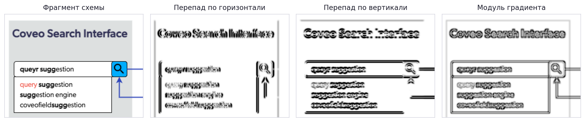
Canny is the next step, which turns the blurry map of changes into crisp outlines. Sobel answers honestly but sloppily. Around every edge it produces a wide band where the change is "fairly strong," and it's unclear where exactly the line runs. Canny first blurs the image slightly so that individual noisy pixels don't pretend to be edges, then walks along each such band and keeps only its ridge, that is, the points where the change is stronger than in their neighbors across the edge. Everything else is suppressed, and the band slims down to a thread. Then points with a change above the upper threshold are declared edges unconditionally, points below the lower threshold are discarded, and those in between are kept only if they touch already accepted ones. Thanks to this, a weak part of a line that wouldn't pass on its own survives because it holds on to a strong one, while a lone speck of noise with the same brightness disappears because it has nothing to hold on to. The output is no longer a gray map but a black-and-white drawing of thin connected lines.
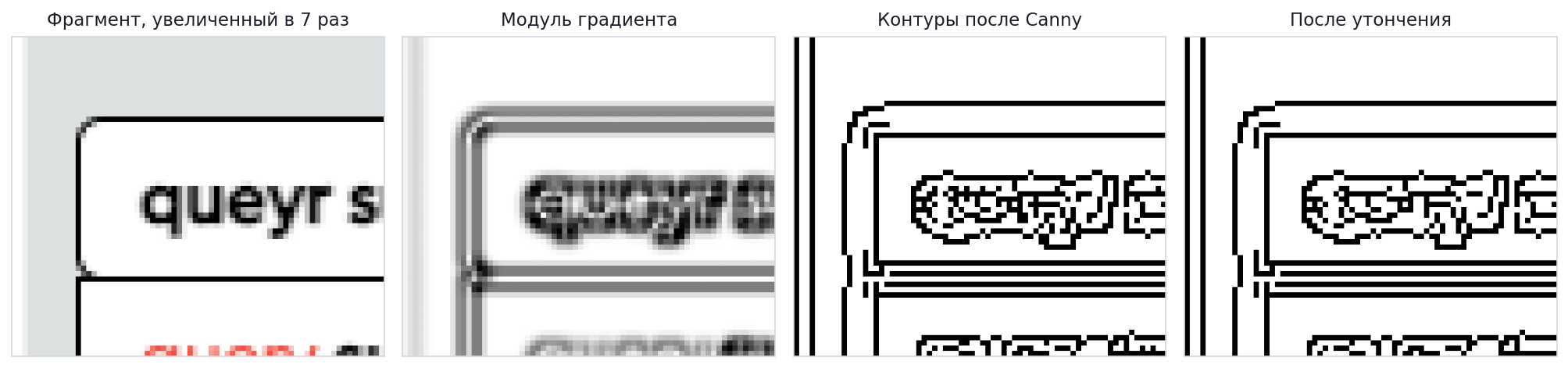
Small connected components with an area under 100 pixels were discarded as text. Then morphology was used to find the diagram's "grid." It's needed so that the final diagram looks neat. Converting from raster always makes things "jump around," and you need to snap them to a grid where possible.
This uses approaches that are formally called erosion and dilation. In this particular case, with a kernel cols // 40 wide, which keeps only long horizontals, and a kernel rows // 40 tall, which keeps only verticals.
These two fancy words are the simplest operations on a black-and-white image, and together they work as a shape sieve.
With erosion, you take a "kernel," in our case a strip one pixel tall and one-fortieth of the image width long (for a 1024-pixel image, that's 25 pixels). Erosion places this strip at every point and keeps the point filled only if everything under the strip is filled. A horizontal line longer than 25 pixels passes this test, although it gets shortened at the ends. But a letter, a vertical line a couple of pixels thick, or a speck of noise disappears entirely, because the strip doesn't fit inside them anywhere.
Dilation does the opposite. It fills a point if there's at least one filled pixel under the strip, and in doing so it grows back the ends of the surviving lines that were eaten away. What has disappeared won't come back, since there's nothing to grow it from.

In the end, only long horizontals remain in the image. Then the strip is turned vertically, one-fortieth of the image height tall, and the same method yields only the long verticals. Dividing by forty instead of using a fixed number of pixels is needed so that "long" means the same thing on a small image and on a large one.

Using the grid coordinates found, a row-by-row pass over the pixels extracted segments even where the Hough algorithm didn't see them. Then came merging collinear segments, with a check that the gap between them doesn't run inside a block and doesn't cross empty space longer than 15 pixels.
What's Hough? It's simple. The Hough transform is a way to find straight lines in an image by voting. You can draw any number of lines through a single filled point, and the point by itself doesn't know which one it lies on. So it votes for all of them at once. Each line is described by two numbers, its angle and its distance from the corner of the image, and a table of counters is set up for all possible pairs. The point goes through angles in steps of, say, one degree, computes for each one at what distance a line with that slope would pass through it, and adds one to the corresponding cell. Once all the points have voted, peaks show up in the table. If a hundred points really lie on one line, all hundred voted for the same cell, while the rest of their votes got spread thinly across the table. Cells with more votes than a threshold are declared detected lines.
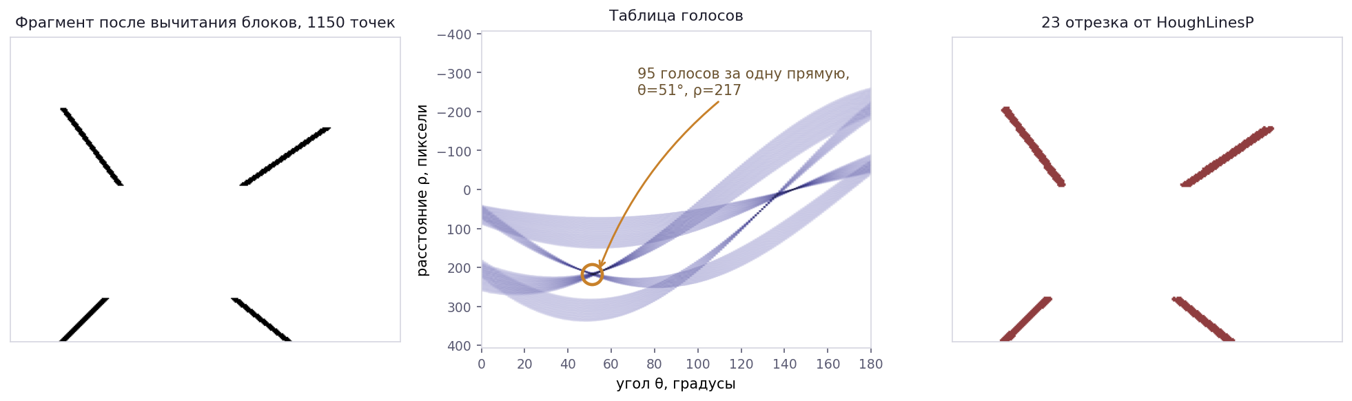
The beauty of the method is that gaps don't bother it. A dashed line or a line crossed by text collects votes just like a solid one. Its weakness is that a short segment collects few votes and sinks below the threshold, while a thick or slightly uneven line splits its votes between neighboring cells and may also fall short. Those are exactly the places where the row-by-row pass over the grid found what Hough didn't see.
The classic version returns infinite lines, with no start and no end. That's why OpenCV users usually go for HoughLinesP, the probabilistic version. It votes with a random sample of points rather than all of them, and once it finds a line, it walks along it in the image and returns concrete segments with endpoint coordinates. It has two parameters: the minimum segment length and the maximum gap that still counts as the same line.
And finally, synthesizing rectangles: iterating over pairs of horizontals and pairs of verticals and checking that all four corners meet:
G = min(w, h) * 0.15
d_tl = dist(v1['p1'], h1['p1'])
d_bl = dist(v1['p2'], h2['p1'])
d_tr = dist(v2['p1'], h1['p2'])
d_br = dist(v2['p2'], h2['p2'])

if max(d_tl, d_bl, d_tr, d_br) <= G:
    # four segments meet at the corners, so treat it as a rectangle
The output was an SVG of lines and rectangles: a vector image that still wasn't a diagram. No labels, no connections, no knowledge that block A is connected to block B.
So I buried most of it.
Three techniques moved from this prototype into the current code: masking detected blocks before searching for lines, checking that the gap between segments doesn't cross a block, and snapping endpoints to block borders. The rest had to go.
An outline instead of four segments
The next idea is obvious once you've taken your lumps with the previous one: a closed shape already comes out of findContours whole, so there's no reason to assemble it from segments.
The current detector does this:
gray    = cv2.cvtColor(image, cv2.COLOR_BGR2GRAY)
blurred = cv2.GaussianBlur(gray, (3, 3), 0)
thresh  = cv2.adaptiveThreshold(blurred, 255, cv2.ADAPTIVE_THRESH_GAUSSIAN_C,
                                cv2.THRESH_BINARY_INV, 11, 2)
canny   = cv2.Canny(blurred, 30, 100)
binary  = cv2.bitwise_or(thresh, canny)
binary  = cv2.morphologyEx(binary, cv2.MORPH_OPEN, np.ones((2, 2), np.uint8))
For those seeing OpenCV code for the first time, a few words of explanation.
cvtColor converts the image to grayscale. Color isn't needed for finding edges, and one number per pixel is easier to process than three. BGR in the name isn't a typo; for historical reasons, OpenCV stores channels in "blue, green, red" order.
GaussianBlur slightly blurs the image with a three-by-three window so that compression grain and lone noisy pixels don't later turn into false edges. The zero at the end means "pick the blur strength yourself based on the window size."
adaptiveThreshold is an adaptive threshold. A regular threshold compares every pixel with a single number for the whole image and breaks down if the background is lighter in some places and darker in others. The adaptive one compares a pixel with the average over its neighborhood, here an 11 by 11 square, with near neighbors weighing more than distant ones. If a pixel is darker than that average by at least 2, it counts as "ink." BINARY_INV inverts the result: ink becomes white, background black. That's the OpenCV convention, where white means an object and black means emptiness.
Then comes the familiar Canny, with a lower threshold of 30 and an upper one of 100. bitwise_or combines two images: a pixel is white if it's white in at least one of them. And last, morphologyEx is a morphological opening, the same erosion and dilation as in the old prototype, only with a two-by-two kernel. Everything smaller than that little square disappears; everything else keeps its shape.
People often write that an adaptive threshold picks up fills. With an 11 by 11 window, that's not quite true: inside a uniform fill, a pixel equals the average of its neighbors and doesn't pass the threshold. In practice, the threshold picks up strokes, text, and the high-contrast edges of fills, Canny adds the weak edges where there's no fill, and the morphological opening removes the grit.
Then a closing with a 5×5 kernel grows over the gaps, and findContours runs on the resulting image.
What's a closing? The next step is to patch up the frames. After the threshold and Canny, they almost always have little holes one or two pixels wide. In one place the line was faint, in another antialiasing broke it. The eye doesn't notice, but to the algorithm a frame with a hole is no longer a closed shape; its interior merges with the background outside. So all lines are first thickened by a couple of pixels in every direction, and small gaps grow together in the process. Then the lines thin back down by the same amount, but the places that have grown together don't come apart. That's exactly what's called a morphological closing. Its kernel is five by five, so gaps of up to four pixels grow over. After that, findContours comes into play: it walks along the border of every region in the image and returns it whole, as a ready-made list of points along the perimeter. These are the very closed shapes that the old prototype painstakingly assembled from four segments.
Next, each outline is classified using a set of metrics, such as circularity 4πS/P², extent ("area to bounding rectangle area"), aspect ratio, smoothness as the number of outline points per unit of perimeter, the number of vertices after approxPolyDP and after the convex hull, and the deviation of angles from 90°.
If the convex hull has 3 vertices, it's a triangle. If circularity is above 0.8 and the sides are nearly equal, let it be a circle. If circularity is above 0.62 and the outline is smooth, we try to find an ellipse or a cylinder in it. Four vertices, extent below 0.62, sides of the minimum rectangle from 0.55, and we call it a rhombus; if the angles deviate by more than 18 degrees, a parallelogram. In all other cases, we call the shape a rectangle.
Obviously, ML would be the right tool for rules like these, but that's the next stage, someday in the future.
A separate check tells a cylinder (the database icon) from an ellipse. A cylinder's mask width is nearly constant in the middle rows, so rows from a quarter to three quarters of the height are taken, and if the width varies by less than 10%, it's a cylinder. Not a great criterion, but it'll do for a prototype. Again, this is a great direction for ML.
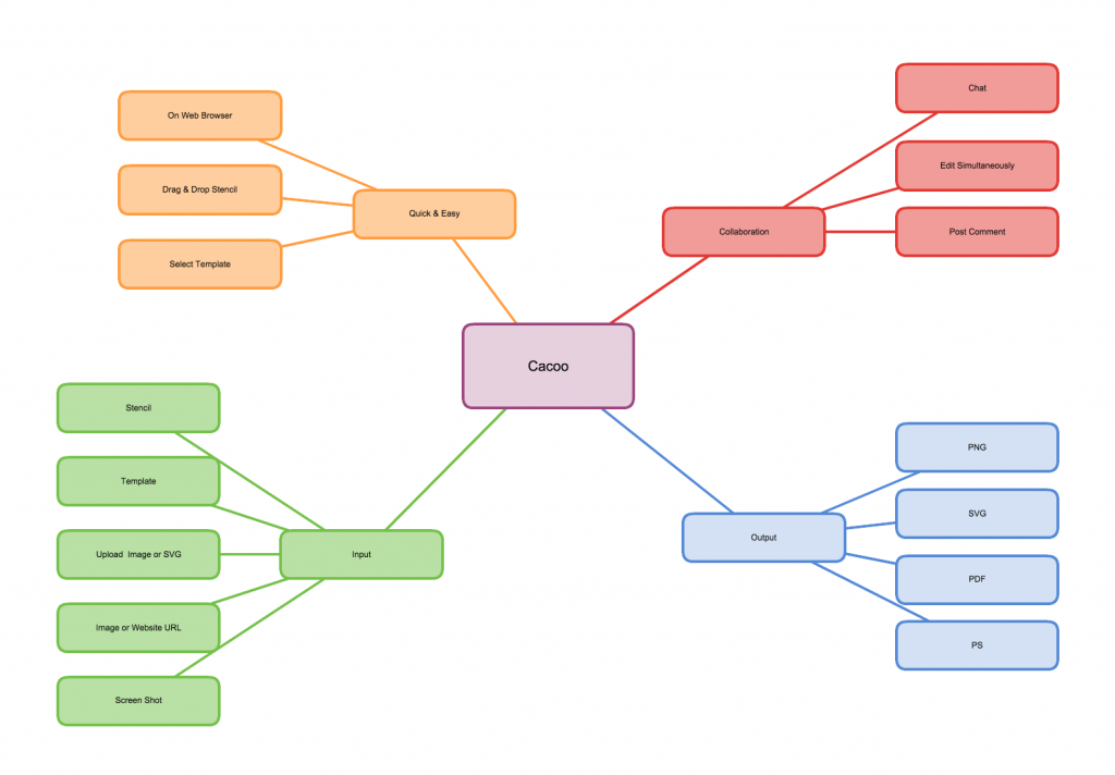
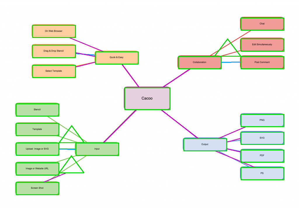
I can show this on two test images. The first is a simple mind map from Cacoo, 1024×712: twenty filled blocks, rounded corners, lines without arrows.
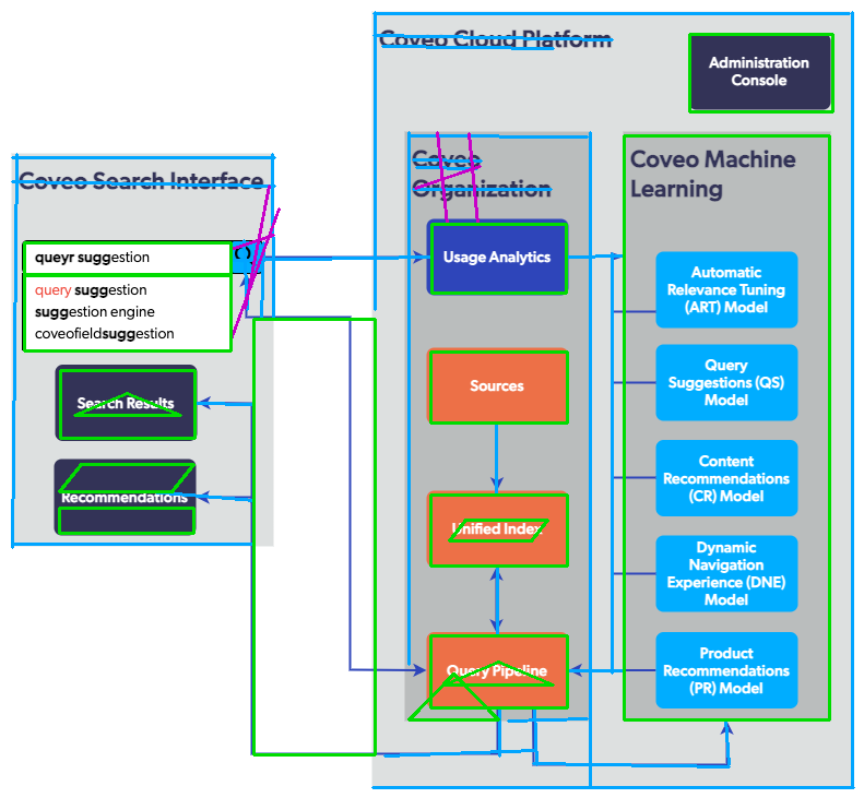
The second is the Coveo architecture diagram, 791×731: nested containers, blocks with multiline labels, arrows with bends, and backgrounds on containers.
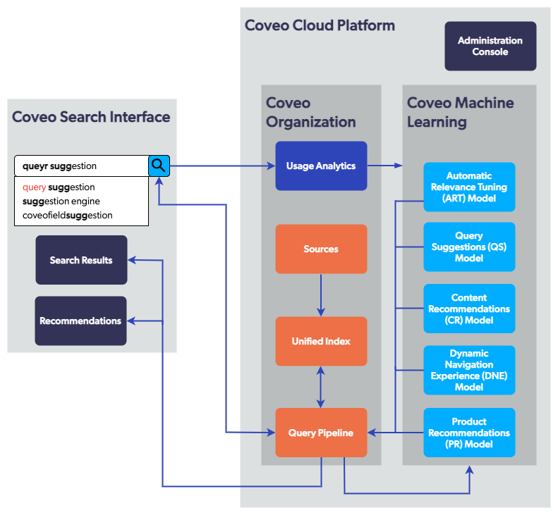
On the first, the detector finds 23 shapes in 7 ms; on the second, 16 shapes in 4 ms. That's on a Core Ultra 9 285K, with no GPU and no network. Not that this is anything special; it's just that everything further down the line that involves the model runs three to four orders of magnitude slower.
Duplicates are removed by IoU with a threshold of 0.5, because a single frame usually produces both an outer and an inner outline.
Holes instead of frames
So I checked connectivity on the Coveo diagram. After the morphological closing, the whole diagram is one connected component. The outer container's frame, the nested block's frame, the arrows between them: all of it is component number one out of eighteen. Lines touch frames, frames touch frames, and the image glues together into one ugly blob.
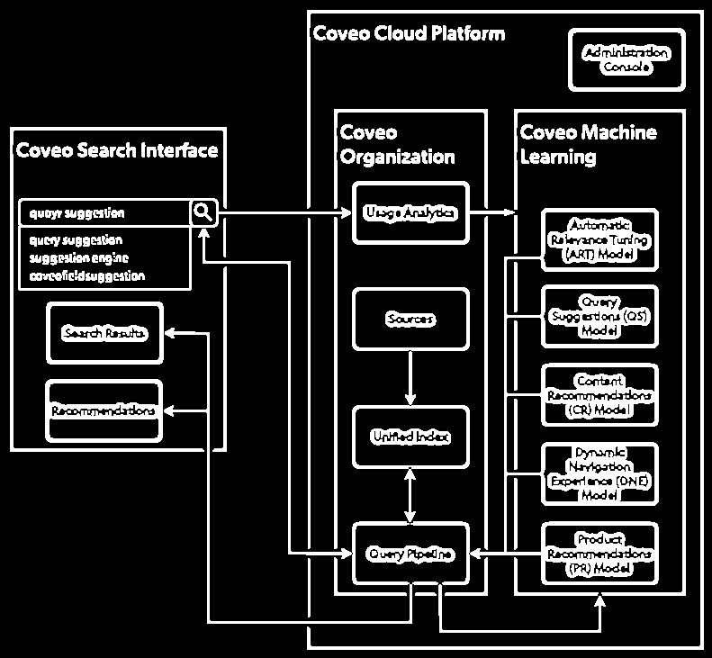
That means blocks don't have separate outer outlines. What reaches the classifier is holes: the white interior of a block, the gray background of a container minus everything nested in it. That's why a block's coordinates are always slightly smaller than the visible ones. The Sources block in the image occupies roughly (390,318)–(521,391), while the detector returns (394,322)–(519,387).
This leads to failures that I had seen before this check but couldn't explain.
First, the largest container disappeared.
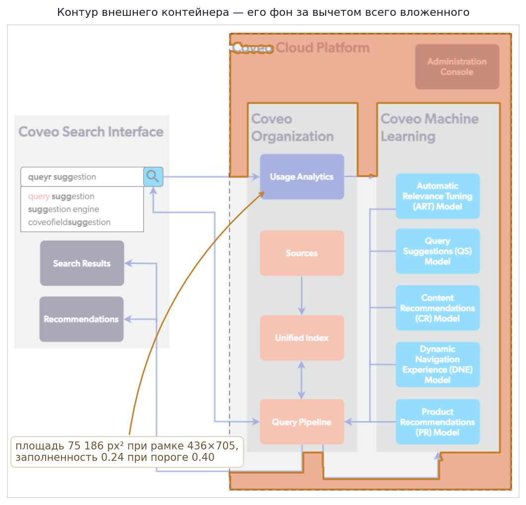
Its hole is the background minus the nested blocks and lines. The area of this shape is 75,186 px² with a 436×705 bounding rectangle, so the extent is 0.24 against a threshold of 0.40. The container is discarded as too full of holes.
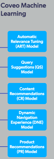
Second, blocks with long text disappear. In the five light blue blocks in the Coveo Machine Learning column, labels of three or four lines reach the edges and cut the hole into strips. Instead of five blocks, the list of outlines holds scraps of their interiors: 123×28 strips with an extent of 0.5–0.64 and five vertices. The "four vertices or convex with an extent above 0.72" check doesn't let them through.
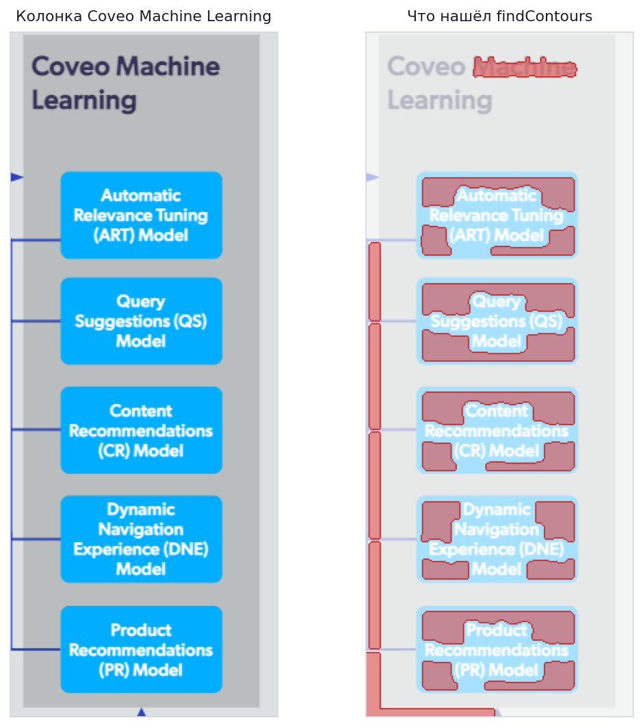
findContours returned in this area. These are pieces of the block interiors, cut up by the lines of the label; none of the five blocks has the outline of its actual frame among them.Third, shapes appear that aren't there. A hole between three intersecting lines is a triangle by every metric, and the classifier records it as a triangle. There are three of these on the mind map, and three more on the Coveo diagram, plus two parallelograms formed out of text.
The result on the Coveo diagram... 16 shapes found: 11 real blocks, three phantom triangles, and two parallelograms. Plus five light blue blocks and the outer container lost.
On the mind map, the result is noticeably better: 20 blocks out of 20, plus three phantom triangles between diverging lines.
Tweaking thresholds doesn't fix this. What's needed is a detector that finds a block by its fill, not by its border. A block's fill is uniform, and the text inside doesn't cut it up. My old prototype, by the way, could find blocks by HSV saturation. I ran it on this same image, and it found exactly three blocks, all dark blue. So simply bringing it back isn't enough.
Segmentation with a neural network
Since classic outlines break down on complex images, it makes sense to try a segmentation model. And I tried two.
Mask R-CNN via detectron2 with COCO weights. The model was trained on photos, and on a diagram it looks for cats, chairs, and people. It produced nothing useful on diagrams, and detectron2 never made it into the project's dependencies.
Segment Anything. This one segments anything, diagrams included. The problem is exactly the opposite. SAM returns every region indiscriminately and doesn't know what a "diagram block" is. For a single image, that's hundreds of masks: frames, fills, letters, pieces of arrows.
So a set of filters sits on top of the masks.
The stability_score, predicted_iou filter has a threshold of 0.88 and cuts off low-confidence masks, which are discarded entirely. The area filter cuts off objects that are too small, unfortunately including text blocks (the setting is 0.2% of the image area). Various rotated regions are cut off as well, because diagrams usually don't have any (yes, that's debatable). A tilt of up to 10 degrees is simply snapped to the axes: diagrams are drawn on a grid, and a couple of degrees usually means antialiasing during rasterization, not the author's intent.
Everything that didn't pass the filters isn't discarded but marked as a fragment. With the --embed-fragments flag, fragments go into the .drawio file as base64 images. The tool won't turn an icon made of three curves into a shape anyway, so let it stay an icon, sitting in the right place.
What computer vision doesn't give you
After the detector, I have coordinates, shapes, and nesting. I don't have the text, the arrow directions, the labels on connections, or the colors named as words.
Classic OCR takes a lot of fiddling here. The text is small, it sits on top of a colored fill, and a block can have three lines with different alignment. And for arrows, there's no classic solution at all: you have to find the arrowhead with a separate detector and match it to the end of a line.
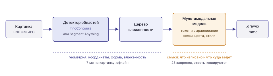
So I handed the semantics over to a multimodal model. In my case, I used Gemini models, but it doesn't really matter; any will do. But I didn't hand over the whole task: asking a model for pixel coordinates of blocks isn't a great idea, because there's nothing to verify them against, they're often hallucinated, and computer vision produces the same coordinates precisely, reproducibly, and for free. The split came out like this: geometry goes to CV, meaning goes to the model.
Three requests per image
In the end, three requests are sent to the model.
The first is OCR, and it sends a crop of a single block, that is, a small piece of the image, which in diagrams is often some block. Besides the text, the model returns how the text is aligned relative to the block, both horizontally and vertically. This is later carried over to draw.io.
The second request is connections. The whole image is sent, and we expect an array of (src, dst, direction, label, style, color) from the model. The third request is styles per block. Each item is (border color, bg color, border style, border width).
For the second and third requests, the image is annotated first. The detected shapes are drawn on top of a copy of the image, and each one's number is written in red at its center. The model receives the image and a list like Box 7: "Usage Analytics" at (55,339)-(178,401), and answers with numbers rather than descriptions. This removes the need to match the answer to the geometry.
The prompt for connections looks like this:
Find all connections (arrows, lines) between boxes. Return a JSON array where each item has:
- "src": source box ID (integer)
- "dst": destination box ID (integer)
- "direction": "forward", "backward", "bidirectional", or "none"
- "label": text label on the arrow/line ("" if none)
- "style": "solid", "dashed", or "dotted"
- "color": one of [black, white, gray, red, green, blue, ...]
How well does it work? On the mind map, the model returned 19 connections, exactly as many as there are edges in a tree of 20 nodes, and the topology matched the image. The central node is connected to four branches, and each branch to its own leaves. All connections have direction: none and empty labels, which is also correct: this diagram has no arrows and no labels.
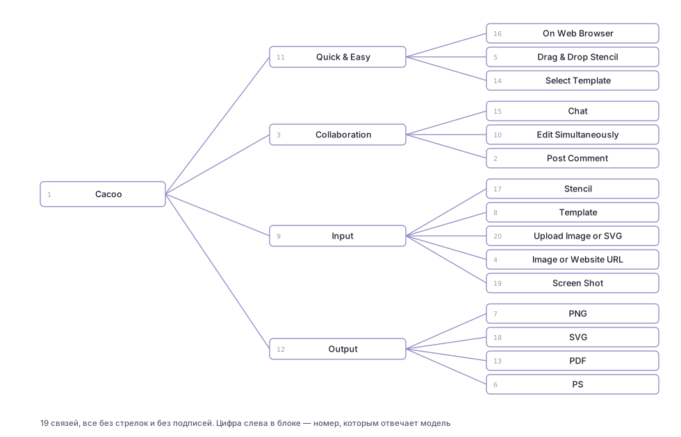
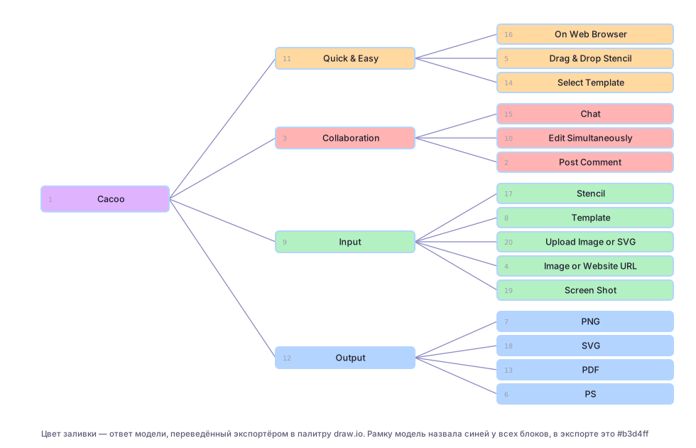
Styles are more interesting. The model returned styles for 21 shapes out of 23, and it named the set of background colors exactly: 6 green, 5 blue, 4 red, 4 orange, and 1 purple, precisely what's drawn, twenty blocks across the branches. The twenty-first shape got white. But it named the border color blue for all 21 shapes, even though each branch of the diagram has its own border color. So the model sees the fill, which covers a large area, but makes up the thin border.
OCR reads text verbatim, author's typos included. On the Coveo diagram, the search field says "queyr suggestion," and that's exactly what ended up in the block label. For reconstruction, that's just what you want.
The model also returns alignment, and it makes it all the way to draw.io. On the Coveo diagram, the container labels are at the top left; the model returned align: left, valign: top, and in the .drawio file the cell got align=left;verticalAlign=top.
The cost. On the mind map with 23 detected shapes, that's 23 OCR requests plus two general ones, so 25 API calls per image. That's why all three steps are cached in temp/: a repeat run on the same image doesn't spend a single request. I haven't yet put all the crops into a single request, although that's the first thing to do for speed.
Why nesting matters
For each block, the tightest block enclosing it is found, and that becomes its parent; a breadth-first traversal from the roots assigns depth. The tree is computed in a single pass and is cheap.
The main consumer of the tree is OCR. A container's crop includes all the nested blocks with their labels, and the model will read them all and glue them into a single line. So before the request, the "children" areas in the crop are whited out, and the model sees only the container's own label.
On the Coveo diagram, this mechanism didn't work, for the reason from the section on holes. The five light blue blocks weren't found, the container has no children, there's nothing to mask, and this crop went into the request:
Also, nesting doesn't make it to the export yet. In .drawio, all cells have parent="1", and Mermaid has no subgraph. The tree exists only for clean OCR, even though the data for real nesting is already computed.
Lines that go nowhere
Geometric connection search is turned on with the --enable-connections flag and works like this.
First, the blocks are subtracted from the binary image. Leaf blocks are covered completely with an 8-pixel margin, while containers get only a 14-pixel-wide strip along the frame; otherwise, all the connections inside a container would disappear along with it. HoughLinesP runs on what's left (remember what that is? scroll back up; you won't forget it now), segments are split into horizontal, vertical, and diagonal ones with a 5-degree tolerance, and collinear ones are merged with a check that the gap doesn't run through a block. Then each segment is checked for coverage. Pixels of the source image are sampled along it, and if less than 4% are filled, the segment is made up. Endpoints snap to block borders within a 60-pixel radius, and duplicates are removed.
On the mind map, 15 segments remain in the end (3 horizontal and 12 diagonal); on the Coveo diagram, 39 (19 horizontal, 14 vertical, 6 diagonal). In the overlays above, these are the purple and light blue lines, and their geometry is correct: the lines run from the edge of one block to the edge of another.
Yet these lines don't make it into .mmd and .drawio. Connections in the export come entirely from the model, while the Hough result is drawn only in the debug images, and that's the project's main open item. The two sources complement each other perfectly: the lines provide the fact of a connection and the attachment points, and the model provides the direction, label, and style. Right now, if the model makes up a connection that isn't in the image, there's nothing to check it against, even though the data for that check is already sitting in the next variable over.
Mermaid and draw.io
Export goes to two formats at once, and they solve different problems.
Mermaid keeps the topology and loses the coordinates. It does the layout itself. A node's shape is encoded in the syntax, and styles in separate directives:
flowchart TD
    box1["Cacoo"]
    box9["Input"]
    box17[("Stencil")]
    box1 --- box9
    box9 --- box17
    style box1 fill:purple,stroke:blue,stroke-width:2px
Draw.io keeps everything else. It's an mxGraphModel with pixel coordinates from the source image, so the result lies right on top of the original. A single block's cell looks like this (the line breaks are mine; in the file it's one line):
<mxCell id="box7" value="Usage Analytics"
        style="rounded=0;whiteSpace=wrap;html=1;fillColor=#b3d4ff;strokeColor=#333333;
               strokeWidth=2;dashed=0;align=center;verticalAlign=middle;"
        vertex="1" parent="1">
  <mxGeometry x="55" y="339" width="123" height="62" as="geometry" />
</mxCell>
The model names a color with a word from a list of twelve names, and the exporter turns the word into a specific pastel shade. yellow becomes #fffacc, cyan becomes #b3f0f0. That's why the output palette looks like the original but doesn't match it. Here's the source diagram and its reconstruction:
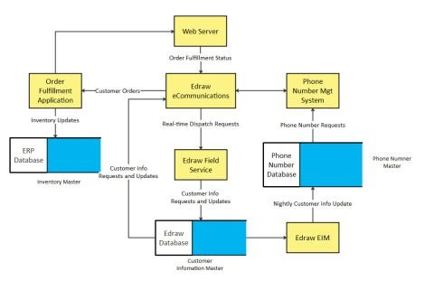
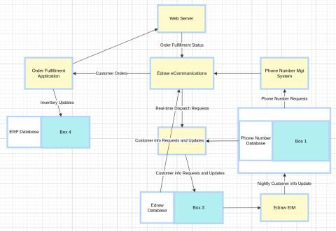
The labels, arrows, and layout were recovered, but the database icons fell apart. A two-tone icon, white on the left and light blue on the right, produces two separate outlines, and the right half remains a rectangle with no text, that is, "Box 4" next to "ERP Database." This is exactly the case that the SAM branch embeds fragments as images for.
The second typical embellishment is overlapping labels on edges. Draw.io places a label at the middle of an edge, and if two edges run side by side, the two labels end up at the same point:
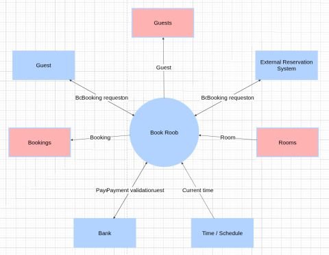
"BcBooking requeston" is "Booking confirmation" and "Booking request" overlapping. The fix is to spread out the attachment points, and the geometry for that, once again, already exists in the Hough lines.
Pitfalls I ran into
A cache keyed by sequence number. The OCR result is stored in the file temp/<image>_box<N>_ocr.json, where N is the block's number in contour traversal order. The order depends on the detector and on the OpenCV version. When I split the monolith into modules, the numbering shifted, but the cache stayed. Today, while writing this article, I finally saw it. The crop diag1_box11.png says "On Web Browser," while the diag1_box11_ocr.json next to it says "Quick & Easy." All the labels shifted onto neighboring blocks, and the export became nonsense, even though both the detector and the model worked correctly. The key should be the crop's content, say its hash together with the coordinates.
Caching errors. If a request fails, {"text": ""} is written to the cache, and the next run takes that emptiness as a ready answer. After problems with the key or the network, you have to delete temp/*_ocr.json by hand. The right thing is not to write the cache when an exception is caught.
Where to get it
Repository: github.com/raliev/diag-vectorizer. You need Python 3.10+, OpenCV, and a Google AI Studio key in the GEMINI_API_KEY variable. The SAM branch additionally requires torch, segment-anything, and the 2.5 GB sam_vit_h_4b8939.pth checkpoint, which goes in the project root.
python -m venv .venv
.venv/bin/pip install -r requirements.txt
export GEMINI_API_KEY=...

# regular run: contours + model
python diag.py input/diag1.png

# plus geometric line search (debug images only for now)
python diag.py input/diag1.png --enable-connections

# SAM branch, embedding unrecognized fragments as images
python diag.py input/diag1.png --algorithm sam \
    --sam-checkpoint sam_vit_h_4b8939.pth --embed-fragments
The output is output/<name>.mmd and output/<name>.drawio, and temp/ holds the crops, debug overlays, and the model response cache. The first thing to open is temp/<name>_overlay.png. It shows right away what the detector found, what it missed, and what it made up, and that explains almost any oddity in the final file.
What's next
The most useful thing in the near term is to bring the geometry and the model together in one place. The Hough lines confirm or refute every connection the model named and provide the attachment points; the model keeps the direction, label, and style.
Next, a detector that finds blocks by fill. That fixes the missing blocks with long text, the missing outer container, and the phantom triangles between lines too.
Then one request instead of twenty-three. Either all crops go to the model in a single message, or the text is read by a local OCR model, leaving Gemini with the arrows and colors.
And nesting in the export: parent on mxCell in draw.io and subgraph in Mermaid. The tree is already computed; all that's left is to write it out.
What's next, part two. Fantasies
Since you've read this far, I'll go ahead and share my vision of the future "at full throttle."
In general, I had a broader idea for an AI tool for diagrams, and everything described above is only the first step toward it.
The idea is that the master document for a diagram, in Confluence or anywhere else, is text. The description can (and should) be fairly detailed, so that the diagram comes out exactly the way the author pictures it. The diagram itself isn't edited directly; only the description is. Well, you can move the circles around, but after that the system has to update the text so that generating from it produces exactly what the user arranged.
The diagram should match the description as closely as possible. If a match can't be achieved (say, a triangle with three obtuse angles simply can't be drawn), the system does the best it can and explains in words what didn't work out. Then the user changes the problem statement until the result suits them.
But there's a trap here: the author may have landed on a good result by accident, with their clumsy text. Regenerate it, and you'll get something different, and not necessarily something good. So you can ask the system to write, from a finished diagram, a description from which the generator will reproduce it exactly. It will be wordier and more layered, but it will reliably lock in the result. What words to use and how much detail is needed for the result to be reproducible is unclear; that's one of the research problems.
From that point on, you're working with text rather than with a diagram. Need a diagram? You compile the text and get what you need. And you don't edit the text by hand either, but through an LLM. Ask it to add a block, and the description changes, but in a way that doesn't suddenly change everything.
The output diagram should be in object form, from which you can then get both a raster (PNG) and a vector (SVG, EPS). It would also be great to feed in existing diagrams or templates, so that the system picks up their styles and established conventions, meaning how to depict what.
Anyway, those are my fantasies. If anyone has an idea of how to build this, let's discuss.
And as for what's already done, feel free to use it, and if you can do better, go for it. That will bring us closer to a real AI diagram editor.
Discussion
Powered by GitHub Discussions — sign in with a GitHub account to join the conversation.