

This is the second article in a series of five on SAP Commerce Order Management. The first one, Order Management Processes That Never Time Out, looked at the process engine underneath OMS and at the ten points where an order waits for a signal from outside. This one goes one layer down, into the step that decides where the goods come from.
The series works at the level of runtime mechanics and project-level configuration decisions, a layer below the task-oriented guides on the SAP Help Portal. Where a mechanism is covered well there, I link to it rather than repeat it, and spend the space on the behavior you have to reason about when you tune the thing.
About the code in this article
The Java snippets below are an illustrative reconstruction: a simplified retelling of the algorithm with renamed variables and collapsed branches, written to communicate what the calculation does. They are not a reproduction of any implementation, and should be read as diagrams. Spring, ImpEx and XSD fragments are different — those are configuration files shipped in the distribution, and I quote them as they are, because the point of a configuration file is that you read and change it.Choosing a shipping location is an assignment problem
A customer orders three items. The retailer holds stock in a national distribution center, four regional warehouses, and two hundred stores that double as fulfillment points. Something has to decide which physical location ships which line, and that decision drives most of the cost and most of the customer experience downstream.
The things the decision trades off are well known across the industry:
- Shipping cost and speed. Closer is cheaper and faster, up to a point. Zone-based carrier pricing makes "closer" a step function rather than a smooth one, so the nearest location is not always the cheapest.
- Package count. Two parcels instead of one roughly doubles the shipping cost and reliably lowers satisfaction. Keeping an order together is often worth a lot of extra distance.
- Inventory health. Shipping from the location with the deepest stock protects the network against stockouts later. Shipping from a location that is about to mark the item down clears aging inventory. These two pull in opposite directions, and which one you want depends on the category.
- Labor. A store that is already handling forty pick tasks today should not get the forty-first, even if it is nearest.
- Business priority. A flagship store, a 3PL with a contractual volume commitment, a warehouse the company wants to wind down.
Approaches to combining these fall on a spectrum. At the simple end are ordered rule lists — "try the pickup store, then the regional warehouse, then the DC" — which are easy to reason about and hard to optimize. In the middle sits simple additive weighting: score each candidate on each criterion, normalize the scores onto a common scale, multiply by weights, and sum. At the complex end are proper solvers, where sourcing is expressed as a mixed-integer program over the whole order and solved for minimum total cost, which is what large retail-specific OMS products do.
SAP Commerce uses simple additive weighting over four criteria, with the weights configurable per base store. For a commerce platform that is a reasonable choice, and the rest of this article looks at how the weighting behaves in practice.
The shape of the sourcing step
Sourcing reads the order and the inventory and produces a plan without writing anything. A separate allocation step turns the plan into consignments and inventory events, which is the subject of the next article.
The steps, in order:
- Order entries are grouped. Entries that must travel together — currently, entries sharing a pickup point of service — form one sourcing context.
- Candidate warehouses are assembled and filtered.
- A sourcing strategy is selected for the context.
- The strategy ranks candidates by fitness and assigns quantities.
- If quantities remain unassigned, the next strategy runs, unless the one that just ran is marked terminal.
Step 2 happens in two separate stages, which is easy to miss when reading the Spring configuration, because the two stages live in different packages and only one of them has "sourcing" in its name.
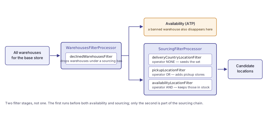
The outer stage is WarehousesFilterProcessor, in the warehouse.filter package. The
reference template gives it a single filter:
<bean id="defaultWarehousesFilterProcessor"
      class="...warehouse.filter.WarehousesFilterProcessor">
  <property name="filters">
    <list>
      <ref bean="declinedWarehousesFilter"/>
    </list>
  </property>
</bean>
DeclinedWarehousesFilter removes warehouses that currently hold a SourcingBan. A ban is
created when a warehouse declines a consignment; the duration for the "too busy" reason is a
property, defaulting to one day:
warehousing.ban.toobusy.days=1This processor is also wired into the warehouse selection strategy that availability uses. A warehouse that declines a consignment therefore drops out of the ATP calculation as well as out of candidate selection, and the storefront sees the ban as reduced availability. Whether that is what you want depends on your network. In a network of ten warehouses the effect is hard to notice, but with two warehouses a ban halves availability for its duration. It is a one-line change if you want sourcing bans to stay inside sourcing.
The inner stage is SourcingFilterProcessor, and its filters combine with set operators
rather than running as a plain chain:
<bean id="sourcingFilterProcessor"
      class="...sourcing.filter.SourcingFilterProcessor">
  <property name="filters">
    <list>
      <ref bean="deliveryCountryLocationFilter"/>
      <ref bean="pickupLocationFilter"/>
      <ref bean="availabilityLocationFilter"/>
    </list>
  </property>
</bean>
Each filter declares a filterResultOperator:
| Filter | Operator | Effect |
|---|---|---|
deliveryCountryLocationFilter |
NONE |
seeds the set with warehouses serving the delivery country |
pickupLocationFilter |
OR |
unions in the warehouse behind the chosen pickup point |
availabilityLocationFilter |
AND |
intersects with warehouses that actually hold stock |
The first filter in the list must use NONE, because there is nothing yet to combine with.
That ordering requirement is implicit in the configuration rather than enforced by it, so if
you insert a custom filter at the head of the list, give it NONE and move the operator onto
the one that used to be first.
The fitness calculation
Once the candidate set exists, ranking it is one nested loop over a matrix.
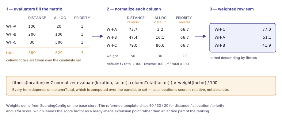
Four factors ship with the reference template, each with an evaluator that produces a raw number and a normalizer that maps it onto 0–100:
| Factor | Default weight | Raw value | Normalizer |
|---|---|---|---|
DISTANCE |
50 | kilometers to the delivery address | reverse |
ALLOCATION |
30 | total available units across the group's products | default |
PRIORITY |
20 | Warehouse.priority, an integer |
reverse |
SCORE |
0 | Warehouse.score, a double |
default |
Weights live on a SourcingConfig attached to the base store, which means they are per-store
and changeable at runtime without a deployment. You will come across other illustrative
splits in SAP's guides and in project templates; what counts is the value in your own
SourcingConfig row, and any default is a starting point. SCORE ships with weight 0: the
factor is wired end to end and stays inert until a project feeds Warehouse.score from
whatever external performance signal it has.
The two normalizers are one line each:
// illustrative
double normalizeDefault(double value, double columnTotal) {
    if (Double.isNaN(value) || Double.isNaN(columnTotal)) {
        return 0d;
    }
    return value / columnTotal * 100d;
}

// illustrative
double normalizeReverse(double value, double columnTotal) {
    if (Double.isNaN(value) || Double.isNaN(columnTotal)) {
        return 0d;
    }
    return 100d - value / columnTotal * 100d;
}
"Default" means bigger is better, "reverse" means smaller is better. Distance and priority use the reverse form, which is why priority 1 outranks priority 5.
And the ranking itself:
// illustrative
double[][] matrix = new double[locations][factors];
double[] columnTotal = new double[factors];

// pass 1 - evaluate, accumulating a total per column
for (int l = 0; l < locations; l++) {
    for (int f = 0; f < factors; f++) {
        matrix[l][f] = evaluatorFor(f).evaluate(location(l));
        columnTotal[f] += matrix[l][f];
    }
}

// pass 2 - normalize against the column, then weight and sum
for (int l = 0; l < locations; l++) {
    double fitness = 0d;
    for (int f = 0; f < factors; f++) {
        double norm = normalizerFor(f)
                .normalize(matrix[l][f], columnTotal[f]);
        fitness += norm * weightOf(f) / 100d;
    }
    result[l] = withFitness(location(l), fitness);
}

sortDescendingByFitness(result);
Adding a factor takes a new evaluator bean, a map entry and a weight column. The next two sections cover the properties of this formulation that produce surprising results on real data.
Fitness is relative to the candidate set
Normalization divides by the column total across the candidates present in this run. A location's score is therefore a share of the column, and it changes when the set of candidates changes.
Most of the time this is invisible, because adding or removing a candidate scales all scores in a column by the same factor and the ordering survives. It stops being invisible when two factors' totals move by different proportions, because the gap between two locations shrinks faster in one column than the other.
Take an order with two lines, five units each, sourced by NoSplittingStrategy, which looks for a single location that can cover everything.
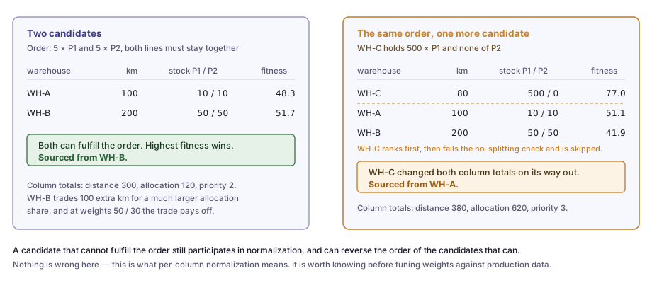
With two candidates, WH-B wins: it is 100 km farther away, but it carries five times the stock, and at weights 50 / 30 the allocation advantage outweighs the distance penalty.
Now a third warehouse joins the candidate set. WH-C is nearby and holds 500 units of the first product and none of the second, so it cannot fulfill this order on its own. The strategy will rank it, discover it fails the no-splitting check, and skip it. But it has already contributed to both column totals — a small amount to distance, a very large amount to allocation. The allocation gap between A and B is compressed much harder than the distance gap, and WH-A now wins.
This is how per-column normalization works in any simple-additive-weighting model, and it affects how you tune one.
Tuning weights against aggregated production data is less reliable than it looks, because the same weights produce different rankings depending on how many candidates happened to clear the filters for a given order. When you tune, hold the candidate set fixed and vary one factor at a time.
Filters also take part in the scoring. A filter that
removes an implausible candidate improves the ranking of everything else, which makes
tightening SourcingFilterProcessor a cheaper lever than re-weighting.
If relative scoring is not what your business wants, you can supply your
own FitnessNormalizer that maps a raw value onto an absolute scale — kilometers against a
fixed 500 km ceiling, say — and register it in fitnessNormalizerMap for the factors you care
about. The normalizer receives the column total and is free to ignore it.
How the distance factor works
The value is a great-circle distance in kilometers, computed with the haversine formula against
an Earth radius of 6372.8 km. It ignores roads and travel time. For dense
urban areas, and anywhere rivers, mountains or borders get in the way, the error is systematic
and in one direction. Projects that care about this typically replace DistanceEvaluator with
one that calls a routing service and caches aggressively, since the evaluator runs once per
candidate per sourcing attempt.
Before distance can be computed, the delivery address needs coordinates. They are written by
GeocodeShippingAddressAction, a step in the order process that runs just before sourcing and
is skipped entirely for pickup orders. It delegates to the geoServiceWrapper bean.
The reference implementation behind that alias is a mock that returns coordinates for any address without reporting an error:
<alias alias="geoServiceWrapper"
       name="defaultCommerceMockGeoWebServiceWrapper"/>
<bean id="defaultCommerceMockGeoWebServiceWrapper"
      class="...storelocator.impl.CommerceMockGeoWebServiceWrapper">
  <property name="baseStoreService" ref="baseStoreService"/>
  <property name="countryIsoGPSLocationMap"
            ref="countryIsoGPSLocationMap"/>
</bean>
countryIsoGPSLocationMap holds nine country entries — CN, JP, US, GB, GG, IM, JE, DE, CA —
plus a DEFAULT of latitude 0, longitude 0. Every address in a listed country geocodes to the
same fixed point for that country; every address anywhere else geocodes to the Gulf of Guinea.
So on a freshly installed system, the distance factor measures the distance from each warehouse
to one of ten fixed points on Earth. Every order shipping to the same country produces the same
distance ranking regardless of the actual address. This behaves well enough for a demo and for
integration tests, and wiring a real geocoder is a documented and straightforward step — the
GoogleMapsServiceWrapper alias swap is a two-line change. I mention it because
sourcing results look entirely plausible before you make that change, so it is easy to leave
for later and then spend a day puzzling over why the nearest store never wins.
One missing coordinate takes out the whole factor
The second distance behavior applies to every other factor too.
DistanceSourcingLocationPopulator sets the distance to null under five separate conditions:
the order has no delivery address; the warehouse has no point of service; the point of service
has no address; the order address has no latitude or longitude; the point of service has no
latitude or longitude. Each writes an INFO line and moves on.
// illustrative
if (deliveryAddress == null) {
    log.info("no delivery address; distance is null");
    target.setDistance(null);
    return;
}
PointOfServiceModel pos = posSelection.get(order, warehouse);
if (pos == null || pos.getAddress() == null) {
    log.info("no usable point of service; distance is null");
    target.setDistance(null);
    return;
}
// ... latitude and longitude checks in the same shape ...
target.setDistance(haversine(posLat, posLon, addrLat, addrLon));
DistanceEvaluator turns that null into Double.NaN. The
first pass adds every raw value into a column total, so a single NaN makes the entire column
total NaN. The second pass hands that total to the normalizer, which returns 0 whenever
either argument is NaN — for every row, including the ones with a valid distance.
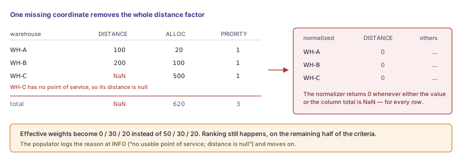
The effective weights become 0 / 30 / 20. Sourcing still produces a plausible answer with normal log output, but for that order it ignores distance. A pure distribution center with no point of service attached is enough to trigger it, and so is one store whose address was imported without coordinates.
The same mechanism applies to the other factors. Warehouse.priority is an Integer with no
default value, so a warehouse created through ImpEx without an explicit priority has null
there and removes the priority factor from every order it is a candidate for.
Warehouse.score does default to 0, so it is safer, but a project that populates it from an
external feed can reintroduce the same hole.
On a project that relies on sourcing, I would add a data check to the deployment pipeline:
every warehouse that can be a sourcing candidate has a point of service with coordinates and a
non-null priority. I would also add custom evaluators
that substitute a defined fallback rather than returning NaN — a large distance for an
unknown location, a middling priority for an unset one — so that a data gap degrades one
candidate instead of one criterion.
The allocation factor measures stock depth
AllocationFitnessEvaluator sums, over every order entry in the sourcing context, the
available quantity of that entry's product at the location:
// illustrative
double evaluate(SourcingLocation location) {
    long total = 0L;
    for (AbstractOrderEntryModel entry : contextEntries(location)) {
        Long available = location.getAvailability()
                                 .get(entry.getProduct());
        total += (available == null) ? 0L : available;
    }
    return (double) total;
}
It is a depth-of-stock measure, paired with the default normalizer, so more is better. The business reading is "prefer the location that is least likely to run out", which is a defensible default for a network where you would rather protect the long tail than clear it.
The name suggests something else, so to be explicit: the factor does not measure how much of this order a location can cover, or how much would be left unassigned. A location holding 1,000 units scores far above one holding exactly the 10 that the order needs, even though both cover the order completely. Summing across entries rather than taking a minimum has the same effect: a location deep in one product and empty in another can outscore a location that holds a little of everything.
Whether that is the right objective is a business question, and the answer differs by category.
If you want coverage rather than depth, the change is small and self-contained — a custom
evaluator returning the unassigned remainder, registered in fitnessEvaluatorMap for the
ALLOCATION key:
// illustrative - lower is better, so pair with the reverse
// normalizer when you register it
double evaluate(SourcingLocation location) {
    long shortfall = 0L;
    for (AbstractOrderEntryModel entry : contextEntries(location)) {
        long needed = unallocatedQuantity(entry);
        long available = availabilityOf(location, entry);
        shortfall += Math.max(0L, needed - available);
    }
    return (double) shortfall;
}
An evaluator where lower is better needs the reverse normalizer, and fitnessNormalizerMap is
keyed by factor, so change both entries together, otherwise the factor inverts. Custom factors
most often go wrong here: an inverted factor throws no exception and ranks the worst candidate
first.
Sourcing strategies and the terminal flag
A sourcing strategy decides how the ranked candidates turn into assignments. The reference template ships three.
NoSplittingStrategy ranks the candidates, then takes the first one that can cover every
line in the group in full. If none can, it assigns nothing and marks the result incomplete.
// illustrative
List<SourcingLocation> ranked = fitnessService.sortByFitness(ctx);
ranked.stream()
      .filter(loc -> coversEveryLine(ctx.getOrderEntries(), loc))
      .findFirst()
      .ifPresent(best -> ctx.getResult().getResults()
              .add(resultFactory.create(ctx.getOrderEntries(), best)));
ctx.getResult().setComplete(isFullyAssigned(ctx));
NoRestrictionsStrategy walks the ranked list in order and takes what it can from each
location until the order is covered. This is a greedy pass with no global
objective, and the number of shipments follows from the ranking.
The two run in sequence, NoSplittingStrategy first, which is how the reference template
expresses "prefer one parcel, accept several". If keeping an order together matters more than
anything else to your business, note that this preference has no weight attached
to it and is expressed only by list order. A project that wants a tunable trade-off needs a strategy that costs
splits explicitly.
PickupStrategy handles click-and-collect. It is selected by a mapper rather than by list
position:
<bean id="pickupSourcingStrategyMapper"
      class="...strategy.mapper.impl.PickupSourcingStrategyMapper">
  <property name="strategy" ref="pickupSourcingStrategy"/>
</bean>
The mapper matches when every entry in the context has a deliveryPointOfService. The logic
is then trivial, because the customer already chose the location.
The bean also sets a property the other strategies leave at its default:
<bean id="defaultSourcingPickupStrategy"
      class="...sourcing.strategy.impl.PickupStrategy"
      parent="abstractSourcingStrategy">
  <property name="posSelectionStrategy" ref="posSelectionStrategy"/>
  <property name="terminal" value="true"/>
</bean>
terminal="true" stops the strategy chain. If the chosen store is short, the strategy assigns
what is there, marks the context incomplete, and no further strategy runs. A pickup order is
never re-sourced to a different location. I think that is the correct default, since a customer
who chose a store to walk into does not want their order shipped from elsewhere without being
asked.
It does mean that partial pickup fulfillment becomes a business process question instead of a sourcing one. The remainder sits unallocated until somebody or something acts on it, and deciding what that is — notify and wait, offer a split, convert the remainder to shipping — belongs on the project's design checklist. The reference template leaves this open, and it is easy to overlook when going live with the template unchanged.
A checklist before going live
The project-level decisions from this article:
| Area | Decision to make |
|---|---|
| Geocoding | replace the mock wrapper; verify coordinates land on addresses, not country points |
| Warehouse data | every candidate has a point of service with coordinates and a non-null priority |
| Factor fallbacks | custom evaluators return a defined value instead of NaN |
| Weights | set SourcingConfig per base store from your own cost model, not from any default |
ALLOCATION semantics |
confirm depth-of-stock is the objective you want, not coverage |
| Sourcing bans | decide whether a declined warehouse should also drop out of ATP |
| Filters | tighten SourcingFilterProcessor, since filters affect scores as well as membership |
| Pickup shortfall | define what happens to the remainder when a pickup store is short |
| Split cost | if parcel count matters, give it an explicit cost instead of relying on strategy order |
Most of these are configuration changes or small beans; the engine itself can stay as it is.
Next in this series (I don't know how soon..): available to promise without a reservation. The ATP calculation is assembled by reflection from a formula item whose boolean properties are matched against DAO method names, and the quantities that drive order state — allocated, shipped, pending, unallocated — are dynamic attributes, which has a direct consequence for anybody trying to report on them in SQL.
Discussion
Powered by GitHub Discussions — sign in with a GitHub account to join the conversation.