
Part 1. The problem
Where the junk in an index comes from
A typical situation: there is a search index filled by a crawler. Hundreds of thousands or millions of pages; the HTML markup has already been stripped from each one, and only the text is left. That text gets indexed, relevance is computed on it, snippets are cut from it, and in recent years it has also been split into chunks for embeddings and RAG.
The problem is that a large part of this text is not content. It is:
- the site template: menus, breadcrumbs, the footer, "© 2024 Company. All rights reserved," social media links;
- service blocks: the cookie banner, "Subscribe to our newsletter," "We use cookies to…";
- legal disclaimers: "The information on this site does not constitute a public offer," "Prices and availability may vary," "Consult a specialist before use";
- blocks the CMS inserts into the article body: "Read also," captions for standard widgets, the same "about the company" paragraph at the end of every news item.
Some of this is cut away by DOM heuristics during parsing. But only some: a disclaimer an editor pasted into the body of every article is, as far as the markup is concerned, indistinguishable from content. And if the index was built long ago, by different parser versions, from different sites, nobody really knows anymore what is left in it.
Why it hurts
It is not just disk space.
- Document length. BM25 and nearly all of its relatives normalize term weight by document length. A page with a short product card and a long footer gets "penalized" for the footer.
- Snippets. If a query happens to match words from a disclaimer, the snippet shows the disclaimer.
- Embeddings and RAG. A chunk that is one-third "We use cookies…" gets a vector that pulls it toward every other such chunk. For vector search, all pages of a site start to look a little alike.
- Deduplication and near-duplicate detection. Two different product cards that share 80% of their template look like near-duplicates.
- Model training. For LLMs this is a known problem: models memorize repeated
fragments of training data verbatim. In the
Colossal Clean Crawled Corpus, a cleaned snapshot of Common Crawl that was used to train
T5 and many other models, researchers found
a 61-word English sentence repeated more than 60,000 times.Lee, Katherine; Ippolito, Daphne; Nystrom, Andrew et al. — Deduplicating Training Data Makes Language Models Better (ACL 2022, arXiv:2107.06499). Exact substring deduplication via a suffix array: the same class of problem as ours, just with a different goal.
So the question that started it all was simple: how much of this junk is in our index, and what are these fragments? Not "how do we cut it out," but first just to see it.
Why not DOM heuristics
The classic answer to "how do I remove boilerplate" is analyzing a single page: text density in a block, link ratio, paragraph length, position in the DOM. This is what Boilerpipe, jusText, Trafilatura, and their descendants are built on.
This approach has two limitations that are fundamental for our problem:
- It looks at one page. It does not know that a paragraph that looks like normal text repeats verbatim on another 40,000 pages.
- It needs markup. And the index no longer has markup, only text.
A definition that works without markup and without knowledge of any particular site goes like this: junk is what repeats. Not individual words (the word "and" repeats too), but long fragments that occur verbatim in many different documents. That is exactly what we will be looking for.
The idea is not new: search engines have been looking for recurring fragments in document collections since at least the mid-2000s.
Part 2. The formulation
Before choosing an algorithm, we need to state precisely what we are looking for. Every word in the definition below will later echo in the algorithm's complexity.
Documents and tokens
A document is a sequence of tokens. Tokenization is as simple as it gets: lowercase
everything and split on anything that is not a letter or a digit. Punctuation
disappears; "All rights reserved." and "all rights reserved" are the same thing.
Each token is replaced with an integer from a dictionary, so from here on we work
with arrays of int rather than strings.
Phrase
A phrase is a contiguous piece of a document: tokens i through (i+k−1), with no gaps. This matters: "free shipping" and "free … shipping" are different things, and we do not care about the second.
Support: in how many documents, not how many times
The support of a phrase is the number of documents in which it occurs at
least once. We denote it df(P), as in document frequency in search.
Why not the total number of occurrences? Because a phrase repeated 500 times inside one long document (a song's refrain, a repeated table row) is not a template. A template is something that runs across documents.
The threshold σ (sigma) is the minimum support at which a phrase becomes
interesting to us. A phrase with df ≥ σ is called frequent.
Maximality
If the phrase "free shipping on orders over 50 dollars" occurs in 1,000 documents, then each of its pieces ("free shipping," "on orders over," "50 dollars") occurs in at least 1,000 as well. Listing them all is pointless: instead of one finding, we would get dozens of its trimmings.
So we look only for maximal frequent phrases: frequent phrases that cannot be extended either left or right while staying frequent.
In the literature, this is called an MCFP — Maximal Contiguous Frequent Phrase. The task: given a corpus and a threshold σ, find all MCFPs. Usually a minimum length is added as well: phrases shorter than 5–10 tokens do not interest us, even if they are frequent.
A toy example that runs through the whole article
Four "pages" of an online store, σ = 3:
D1: new laptop acer swift free shipping on orders over 50 dollars
D2: case for iphone 15 free shipping on orders over 50 dollars
D3: free shipping on orders over 50 dollars sony headphones
D4: sony headphones wh 1000 free shipping
The answer:
- "free shipping on orders over 50 dollars":
df = 3(D1, D2, D3). Frequent. It does not extend to the left (it is preceded by "swift," "15," and the start of the document), nor to the right. Maximal. - "free shipping":
df = 4. Frequent, even more so. But not maximal: its extension "free shipping on" is also frequent (df = 3 ≥ σ). - "sony headphones":
df = 2 < 3. Not frequent.
Note the second item: the sub-phrase has higher support than the maximal phrase, and it still does not make it into the answer. Maximal does not mean "most frequent"; it means "longest of those still frequent." This will come in handy when we check maximality in the algorithm.
Part 3. From simple to complex
Step 0. Count n-grams
The most obvious solution: pick a length n, slide a window over all documents, put all n-grams into a hash table "n-gram → set of documents," and filter by σ.
For n = 2 on our example:
free shipping        {D1, D2, D3, D4}   df=4  ✓
shipping on          {D1, D2, D3}       df=3  ✓
on orders            {D1, D2, D3}       df=3  ✓
orders over          {D1, D2, D3}       df=3  ✓
over 50              {D1, D2, D3}       df=3  ✓
50 dollars           {D1, D2, D3}       df=3  ✓
sony headphones      {D3, D4}           df=2
new laptop           {D1}               df=1
... another fifteen or so with df=1
It works. There are three problems, and all three lead to the next steps.
Problem 1: which n? A template phrase may be 6 tokens long, or it may be 300 (a whole disclaimer paragraph). A fixed n either cuts long phrases into pieces or misses short ones.
Problem 2: memory. The number of distinct n-grams in natural language grows almost as fast as the number of tokens: starting from n = 3–4, the overwhelming majority of n-grams are unique. On a corpus of 3 billion tokens, that means billions of keys in the hash table, each with a list of documents. No amount of memory is enough, and almost all of it goes to n-grams that occurred once and that we certainly do not need.
Problem 3: trimmings. Even if we try every n, the answer will consist of nested pieces of one and the same phrase. Here is an actual excerpt from the output of my early prototype without a maximality check (the corpus is Java source code, so the "template" here is annotations and imports):
df=2985  len=9  import org springframework beans factory annotation required public class
df=2985  len=8         org springframework beans factory annotation required public class
df=2985  len=7             springframework beans factory annotation required public class
df=2985  len=6                             beans factory annotation required public class
df=2985  len=5                                   factory annotation required public class
Five lines, one finding. That run produced 77,000 such lines.
Step 1. Apriori: grow from frequent to frequent
The key observation the whole field rests on: support is
anti-monotone. If phrase P occurs in a document, every piece of it occurs there
too. Hence, df(piece) ≥ df(P). Corollary: if a short phrase is not frequent,
no phrase containing it is frequent either.
This gives a strategy: start with short frequent phrases and extend only them. A non-frequent extension is discarded along with everything that could have grown from it. This is the idea behind Apriori/GSP, data mining classics from the mid-'90s.
On the example: six of the bigrams are frequent. "sony headphones" is discarded,
which means "sony headphones wh" and everything beyond it need not be examined. And
"free shipping" extends to "free shipping on" (df=3), that to "free shipping on
orders" (df=3), and so on up to "… 50 dollars." There is nothing further to extend
with: on the right, D1 and D2 end, and D3 has "sony," with df = 1.
Problem 1 (which n) is solved: length is no longer a parameter; a phrase grows on its own as long as it stays frequent. Problem 3 (trimmings) is solved by a maximality check on output. But problem 2 (memory) is not: at the first level, we still have to count all bigrams to learn which of them are frequent.
Step 2. Sequential pattern mining: too general a tool
For the task "find frequent sequences," there is a whole family of ready-made algorithms: GSP, PrefixSpan, SPADE, BIDE+, VMSP, CloSpan. Many of them are collected in the SPMF library and are easy to pick up and run.
The catch is that they solve a different, more general problem. In classic
sequential pattern mining, gaps are allowed between the elements of a pattern:
the pattern ⟨A, B, C⟩ counts as present in a document if it contains
A … anything … B … anything … C. For market basket analysis, that is exactly
what you want. For text, it is a combinatorial explosion: in a long document, almost
any three frequent words can be found in the right order somewhere, thousands of
tokens apart. The number of candidates grows by orders of magnitude, and almost all
of them are meaningless.
You can restrict these algorithms to contiguous extensions (SPMF has, for example, a "contiguous" variant of BIDE+), but their internal data structures (projected databases, position lists for every prefix) are designed for the general case and consume memory accordingly. In our benchmarks, all SPMF algorithms (BIDE+, VMSP, GST) ran out of memory already at 1,000 books, which is about 60 million tokens with a 40 GB heap. Billions are far out of their reach.
Takeaway: we need a tool that knows from the start that there are no gaps.
Step 3. Suffix arrays: an exact answer from stringology
The task "find all repeated substrings" is a stringology classic, and it has a classic solution.
A suffix array is all suffixes of a text, sorted lexicographically (what is stored, of course, is not the suffixes themselves but their starting positions). The LCP array next to it stores, for each pair of adjacent suffixes, the length of their common prefix.
Why this solves the problem: in the sorted array of suffixes, all occurrences of any substring lie next to each other: they are the suffixes that start with it. And the LCP array tells you where such blocks begin and end.
A small example. Let's concatenate three documents into one text with separators (letters are tokens):
D1: A B C D D2: X A B C D3: A B C YThe sorted suffixes (only the beginning of each is shown) and the LCP with the previous one:
  #   suffix           doc   LCP
  1   A B C $          D2    —
  2   A B C D $        D1    3
  3   A B C Y $        D3    3
  4   B C $            D2    0
  5   B C D $          D1    2
  6   B C Y $          D3    2
  7   C $              D2    0
  ...
Rows 1–3 form an LCP interval: three adjacent suffixes with a common prefix of
length ≥ 3, that is, "A B C." The suffixes come from three different documents,
so df = 3. Rows 4–6 are the interval for "B C," also df = 3, but "B C" is
contained in "A B C" with the same support, so it is not maximal.
A bottom-up traversal of all LCP intervals (using a stack) enumerates all repeated
substrings, and counting distinct documents in each interval gives df. This is
what the Fischer–Heun–Kramer (FHK) algorithm is built on; it solves the problem
in time that is asymptotically optimal in the input size. There is also an
alternative with top-down traversal and early subtree pruning: DFI (Deferred
Frequency Index).
It is an exact and elegant method. Its problem is the constants. The suffix array and the LCP array each take one integer per token of the corpus, plus the text itself, plus an array mapping each position to its document, plus auxiliary traversal structures. And all of it is built for the entire corpus, including billions of positions where no frequent phrase begins. In our measurements, FHK gets as far as 30,000 books (≈1.7 billion tokens) and runs out of memory beyond that, while DFI, with its sparse table for RMQ, fails already at 5,000.
Stringology answers the question "where does any substring repeat?" We need the answer to a narrower question: "where does a frequent substring repeat?" And most substrings of natural language are not frequent.
Part 4. BloomSpan
The main idea
Let's look at the corpus through the lens of Zipf's law. The distribution of n-grams in natural language is a long tail: the overwhelming majority occur once or twice. This holds for bigrams too. On the Gutenberg corpus at σ = 20, about 2% of all bigrams meet the threshold.
Hence the idea: first cheaply throw away 98% of the corpus, and build the expensive structures only for the remaining 2%.
"Cheaply" here means without storing the n-grams themselves. That is what probabilistic data structures are for.
A Bloom filter with counters
An ordinary Bloom filter answers the question "have we seen this element?" It is a bit array: an element is hashed, and the corresponding bits are set to 1. It can err in one direction: say "yes" about an element that was never added (a hash collision). But it will never say "no" about an element that was.
A Counting Bloom Filter stores small counters instead of bits. To add an element, you increment the counter in the cell it hashes to. To ask "how many times have we seen it," you read the counter.
The property is the same: it only errs upward. If two different bigrams land in the same cell, the counter shows their sum, which is more than either of them. It will never show less than the true count.
A toy illustration: an array of 8 counters, with bigrams hashed into cells.
cell:       0   1   2   3   4   5   6   7
counter:    3   1   4   0   3   2   3   5
                    ↑                   ↑
            "free shipping"       three bigrams landed here:
              (4 times)           "50 dollars"       (3 times)
                                  "new laptop"       (1 time)
                                  "headphones wh"    (1 time)
"new laptop" occurred once, but because of the collision, the filter says "5." At the filtering stage, it will pass as a candidate and be weeded out later, during exact counting. The opposite situation, a frequent bigram for which the filter counted less than σ, is impossible.
Why the filter never loses a frequent phrase
This is the algorithm's central property, and its proof takes three lines.
The filter counts not the document frequency df but the total number of
occurrences c. This is simpler: we do not need to remember in which document we
already incremented the counter. Let ĉ(S) be what the filter shows for n-gram S.
- Collisions only add:
ĉ(S) ≥ c(S). - Every document containing S contributes at least one occurrence:
c(S) ≥ df(S). - Therefore
ĉ(S) ≥ df(S), and ifdf(S) ≥ σ, the filter is sure to show≥ σ.
So every truly frequent n-gram passes the filter. It remains to make sure that all frequent long phrases can be grown from them. This follows from anti-monotonicity: any frequent phrase of length ≥ n contains an n-gram that is frequent as well (with no lower support). So every frequent phrase has at least one "seed" that survived the filter.
There are no false negatives at the selection stage. There are false positives, and quite a few of them: the filter counts occurrences, not documents, so a bigram that occurred 20 times in a single book also passes at σ = 20. The next step, which is exact, weeds them out.
Here is what this looks like in code (the Java implementation, abridged):
// Size: 8 bytes per corpus token, but no more than 512 MB
byte[] filter = new byte[filterSize];

// One linear pass: each bigram increments its counter
for (int p = 0; p <= seq.length - n; p++) {
    int idx = (int) (Math.abs(hashTokens(seq, p, n)) % filter.length);
    int c = filter[idx] & 0xFF;
    if (c < 255) filter[idx] = (byte) (c + 1);   // saturates at 255
}
A couple of engineering details. The hash is FNV-1a over integer tokens. There is only one
hash function, so formally this is a single row of a Count-Min Sketch rather than a "real"
multi-hash Bloom filter; this does not affect the guarantee, only the false positive
rate. Each counter is one byte and saturates at 255; that is why the comparison is
against min(σ, 255), and the "only errs upward" guarantee holds.
A second filter: by individual words
Besides the bigram filter, there is a second, very cheap one: the exact document frequency of each individual token (there are millions of them in the dictionary, not billions, so this is just a hash table). If at least one word of a bigram occurs in fewer than σ documents, the bigram cannot be frequent. Same anti-monotonicity.
A candidate seed passes only if it passes both filters. On the Gutenberg-BookCorpus corpus at σ = 20, together they cut 98% of all bigrams.
Merging seeds and exact support
For the surviving 2%, we can finally afford exactness. Each occurrence of a
candidate is recorded as (bigram, document, position); a bigram of two 32-bit
tokens is packed into a single long. The array is sorted in parallel, and
identical bigrams end up next to each other. One pass over it, and for every
bigram we know the exact list of occurrences and the exact df. Everything with
df < σ is discarded: these are the filter's false positives.
At this stage, we have seeds: frequent bigrams with lists of all their occurrences.
Processing order: the "heaviest" first
Seeds are sorted by the score
Ψ(P) = |P| × df(P)that is, length times support, which is roughly "how many corpus tokens this phrase covers." Ties go to the longer one first, then lexicographically (so that the result is deterministic).
Why: the seeds that will grow into the most massive templates, the "backbones" of the corpus, are processed first. Once such a backbone is found, all of its pieces that show up later will quickly be recognized as already covered.
Depth-first growth directly on the corpus
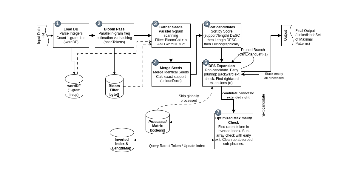
Each seed grows to the right by depth-first search with a stack. For the current phrase, we look at the token following each of its occurrences and group the occurrences by that token. Each group that covers ≥ σ documents is a frequent extension and gets pushed onto the stack.
Where this happens matters: directly in the original token array. No projected
databases, no copies of suffixes: an occurrence is a (document, position) pair,
and the "next token" is simply doc[pos + len].
On the example: the seed "free shipping" (occurrences in D1, D2, D3, D4). The next tokens: D1 → "on," D2 → "on," D3 → "on," D4 → end of document. The "on" group covers 3 documents ≥ σ → "free shipping on" with three occurrences is pushed onto the stack. And so on up to "… 50 dollars," where the next tokens are end, end, "sony," and no group reaches σ. It cannot be extended any further.
Early pruning: if all left neighbors are the same
Before extending a phrase to the right, the algorithm checks one thing: do all occurrences have the same token on the left?
If so, the phrase is certainly not maximal: it can be extended to the left without losing support. And the algorithm will find that longer version anyway, from another seed that starts one token earlier (that seed is frequent too, with the same support). So the current branch can be thrown away entirely, along with everything that would have grown from it.
On the example: the seed "shipping on." All three of its occurrences have "free" on the left. The branch is pruned immediately; the whole phrase will be found from the seed "free shipping."
This is a cheap check (a single pass over the occurrences), and it removes most of the duplicate work: without it, every long template of length L would be "grown" almost L times, once from each of its inner seeds.
Maximality check
When a phrase no longer grows to the right, we need to decide whether it goes into the answer. Two questions:
(A) Is it a piece of an already found phrase? Naively, compare it with all found phrases. That is expensive: there may be tens of thousands of them. So we maintain an inverted index "token → found phrases containing it." For a candidate, we take its rarest token (according to this index), and only need to compare it with the phrases in that token's list. If a super-phrase exists, it must contain this token as well, so nothing is lost, and the list is usually very short.
(B) Does it absorb something found earlier? If the new phrase is longer and contains a previously found one, the old one is removed from the answer and from the index.
This is exactly the situation with "free shipping" from Part 2: a sub-phrase may have higher support, it may be found earlier, and it still has to give way to the super-phrase in the end.
The coverage mask
The last mechanism is a global bitmask the length of the entire corpus: one flag per position. When a phrase is confirmed as maximal, all positions of all its occurrences are marked. If all occurrences of the next seed lie in already-marked positions, it is skipped without even starting to grow.
Thanks to the Ψ ordering, this happens often: backbones are found first, and most of the subsequent seeds are their insides.
This mask has a second purpose, which is more important for the original task than the first. We will come back to it in Part 6.
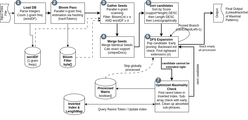
The whole algorithm
- Load the corpus as
intarrays and compute the exactdfof each word. - One linear pass: all bigrams go into the counting filter.
- A second, parallel pass: keep the bigrams that pass both filters.
- Sort the occurrences, merge them, compute the exact
df, and discard false positives. - Sort the seeds by Ψ.
- For each seed (unless it is covered by the mask), grow it depth-first with early pruning.
- Check maximality via the inverted index and update the mask.
What it costs
Let W be the number of tokens in the corpus, M the filter size, C the number of occurrences of surviving seeds, and P the number of phrases found.
Memory: O(W + M + C + P). The corpus and the mask take O(W) each, the filter
takes exactly M bytes (up to 512 MB in our case), and the seeds and the index are
proportional to what survived the filter. The key difference from the suffix array:
the expensive structures are built not for all W positions, but only for C, and
C is a few percent of W.
Time: the filter and seed gathering are linear passes plus sorting the seeds,
Θ(W + C log C). The growth phase depends on the data, and there is no honest
worst-case bound for it. Instead, there are the measurements in the next part.
To be honest about it in brief: in the worst case, BloomSpan is no better than the exact methods, and sometimes worse. It wins on a certain "shape" of data, and that shape is exactly what is typical of natural text.
Part 5. Measurements
How we measured
All algorithms are implemented in Java and were run on the same machine (Intel Core
Ultra 9, 64 GB RAM, OpenJDK 21, heap -Xmx40g). FHK and DFI are in-house
implementations (SA-IS + Kasai's LCP); BIDE+, VMSP, and GST come from SPMF. Time is
measured from the algorithm call to the result, including suffix array construction
for FHK/DFI. Each configuration was run 6 times; the first run is discarded as JVM
warm-up, and the tables show the median of the other five.
Datasets:
| dataset | what it is | σ | min. length |
|---|---|---|---|
| Synthetic 1 | documents made of randomly generated "words" (not English) with three fixed phrases inserted | 3 | 3 |
| Synthetic 2 | 300 heavily overlapping phrases of decreasing length: the worst case for BloomSpan | — | — |
| Gutenberg-8k | 8,544 books from Project Gutenberg, 535 million tokens | 10 | 5 |
| Gutenberg-BookCorpus-Cleaned | up to 50,000 books, up to 3.07 billion tokens | 20 | 10 |
How Synthetic 1 is built. Its "words" are not English words but random
strings: each is 8 random lowercase Latin letters (qhzbtwla, mfoxkrdu, and so
on). The generator works like this:
- Generate N × 5,000 strings of 8 random letters, discarding duplicates, so that all strings are unique across the entire corpus. There are 26⁸ ≈ 2·10¹¹ possibilities, so a real English word among them is a rare accident, and meaningful combinations do not occur at all.
- Slice them sequentially into documents of 5,000 each. As a result, every
background "word" occurs in exactly one document,
df = 1: the background has no repeats by construction. - Take three short English phrases with a given support from a CSV file ("This is the first test sentence": 3 documents, "Another unique phrase for testing": 5, "A third sentence": 4). For each, pick that many different random documents and insert the whole phrase at a random position between background words.
The result is a corpus whose correct answer is known in advance: exactly three
frequent phrases and nothing else. It is a correctness check and a stress test on a
"flat" distribution with no repeats, but such a corpus does not resemble natural
text. The generator is in the repository
(corpus-miner/test-gen/generate_test_dataset.py).
Correctness was checked directly: on Gutenberg-8k, at every size where at least one exact baseline completes (up to 5,000 books), the phrase sets of BloomSpan, FHK, and DFI were sorted and compared, and they match completely. Nothing missing, nothing extra. Beyond 5,000 books, there is nothing to compare against, and no equivalence is claimed there.
The large corpus: what BloomSpan was designed for
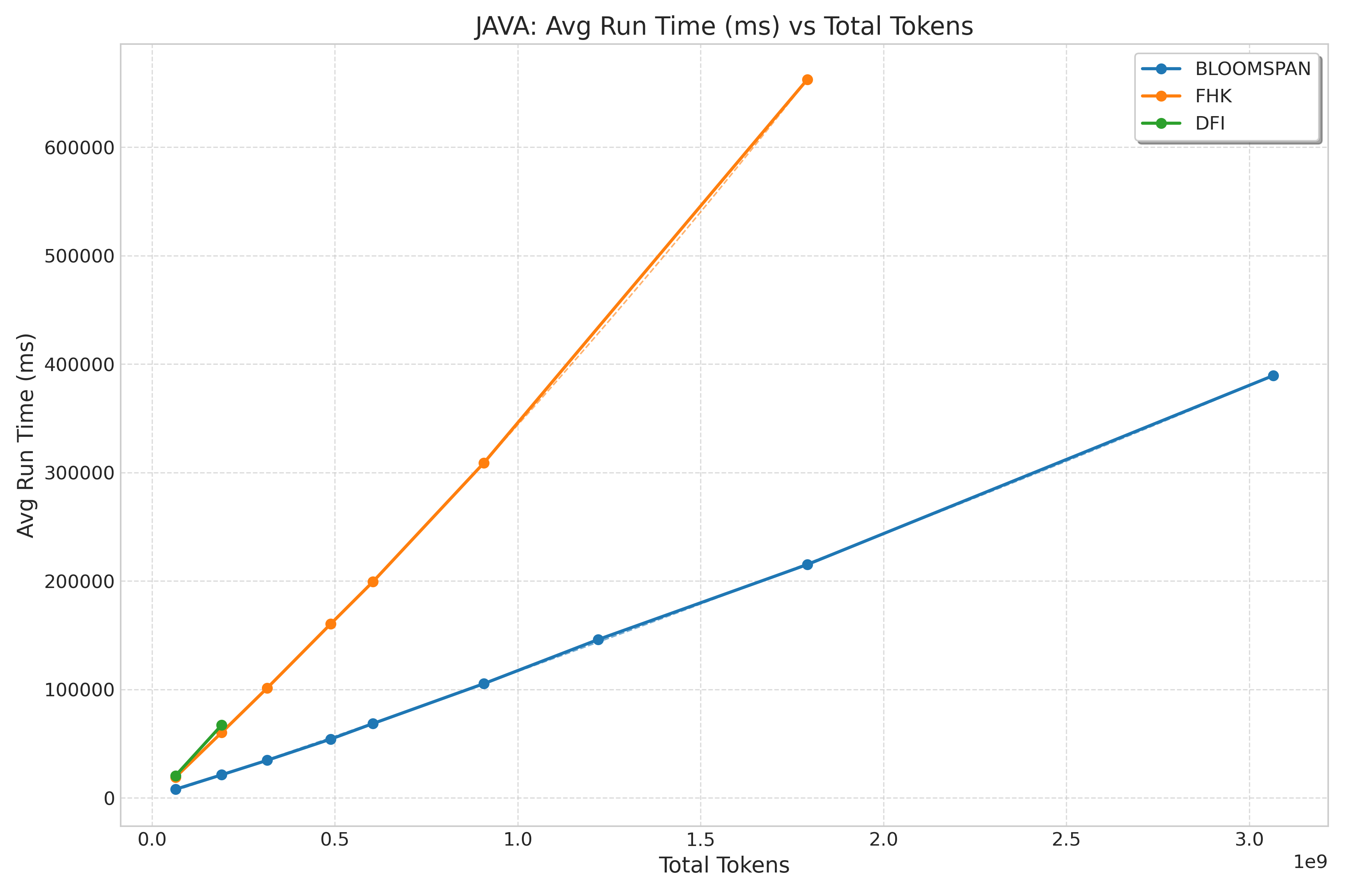
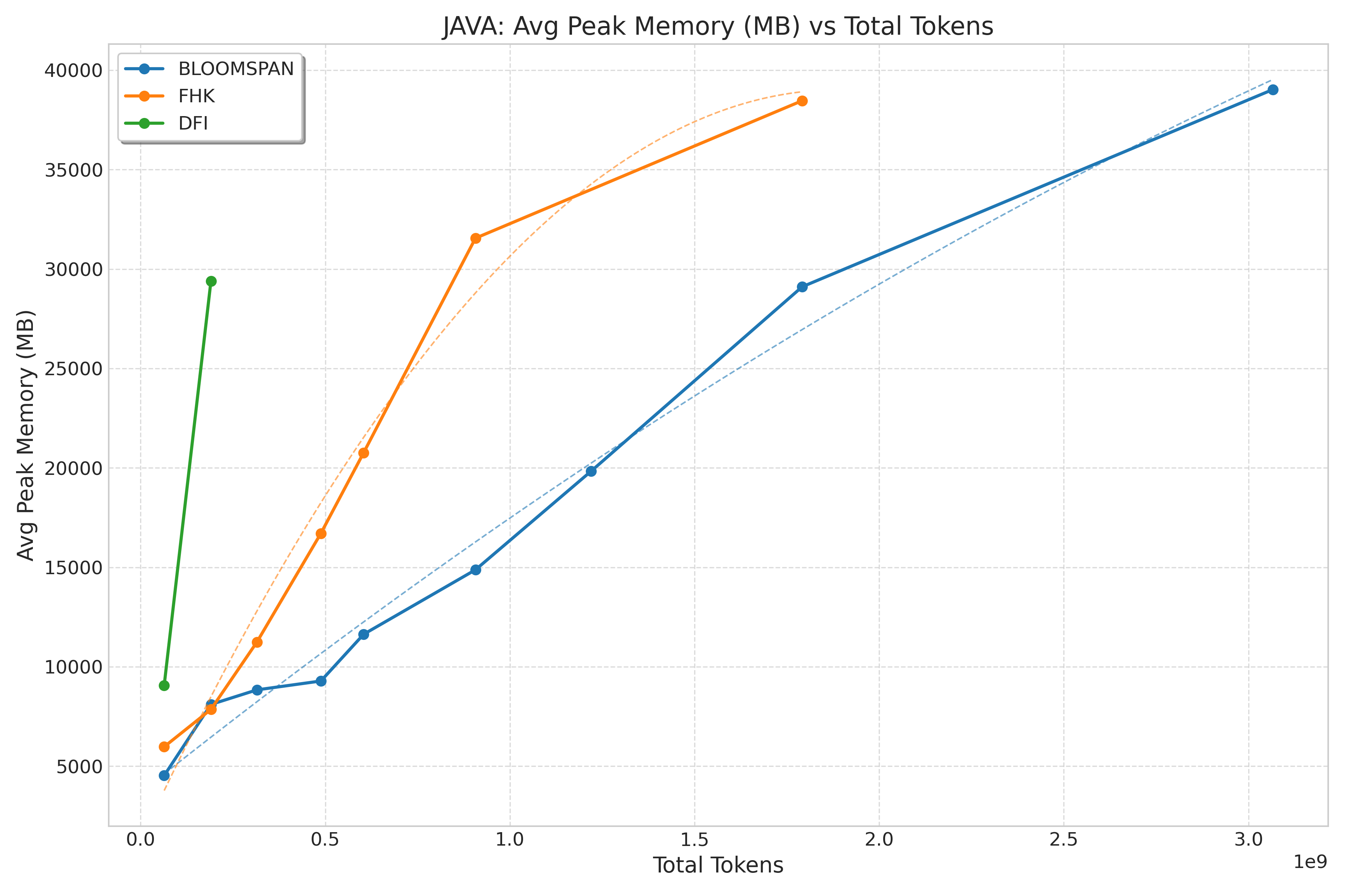
Gutenberg-BookCorpus-Cleaned, σ = 20, minimum length 10. Time in seconds, memory in MB; OOM means 40 GB was not enough.
| books | BloomSpan, s | BloomSpan, MB | FHK, s | FHK, MB | DFI, s | DFI, MB | speedup | phrases |
|---|---|---|---|---|---|---|---|---|
| 1,000 | 1.73 | 5,095 | 19.08 | 6,591 | 20.17 | 9,138 | 11.0× | 31 |
| 3,000 | 4.16 | 7,836 | 60.34 | 7,856 | 67.25 | 29,393 | 14.5× | 120 |
| 5,000 | 6.64 | 6,977 | 101.33 | 11,238 | OOM | OOM | 15.3× | 217 |
| 8,000 | 10.41 | 8,853 | 160.37 | 16,708 | OOM | OOM | 15.4× | 375 |
| 10,000 | 13.59 | 12,044 | 199.34 | 20,764 | OOM | OOM | 14.7× | 516 |
| 15,000 | 20.80 | 14,979 | 308.67 | 31,549 | OOM | OOM | 14.8× | 1,034 |
| 20,000 | 27.67 | 20,839 | — | — | OOM | OOM | — | 1,964 |
| 30,000 | 44.61 | 29,385 | 662.24 | 38,461 | OOM | OOM | 14.8× | 3,673 |
| 50,000 | 383.27 | 38,873 | OOM | OOM | OOM | OOM | — | — |
What we see here:
- 11–15 times faster than FHK at every point where both completed.
- The memory gap grows with size: at 15,000 books, it is 15.0 GB versus 31.5 GB.
- DFI, with its sparse RMQ table (
O(n log n)memory), eats 29 GB already at 3,000 books and fails at 5,000. FHK gets as far as 30,000 books (≈1.7 billion tokens). BloomSpan is the only one that completed 50,000 books (≈3.07 billion tokens) within 40 GB. - Scaling is almost linear: up to 30,000 books, the cost of processing one token stays in the range of 0.021–0.027 µs while the input grows 28-fold. The slope on a log-log scale is 0.98.
- At 50,000 books, linearity breaks: the cost jumps to 0.125 µs per token. The reason: there are now many phrases, and the maximality check, whose cost depends on the size of the answer, comes to the fore. The slope over all nine points is 1.24.
Where BloomSpan loses
It would be dishonest to show only the convenient table. There are three regimes where BloomSpan is not the best.
Synthetic 1 (sparse insertions into a unique background). Up to 10,000 documents, all stringology algorithms scale roughly linearly and stay close. At 12,000 documents there is a crossover, and beyond it FHK is faster and leaner: at 30,000 documents, FHK takes 15.3 s and 38.9 GB, while BloomSpan takes 38.2 s and hits the heap limit.
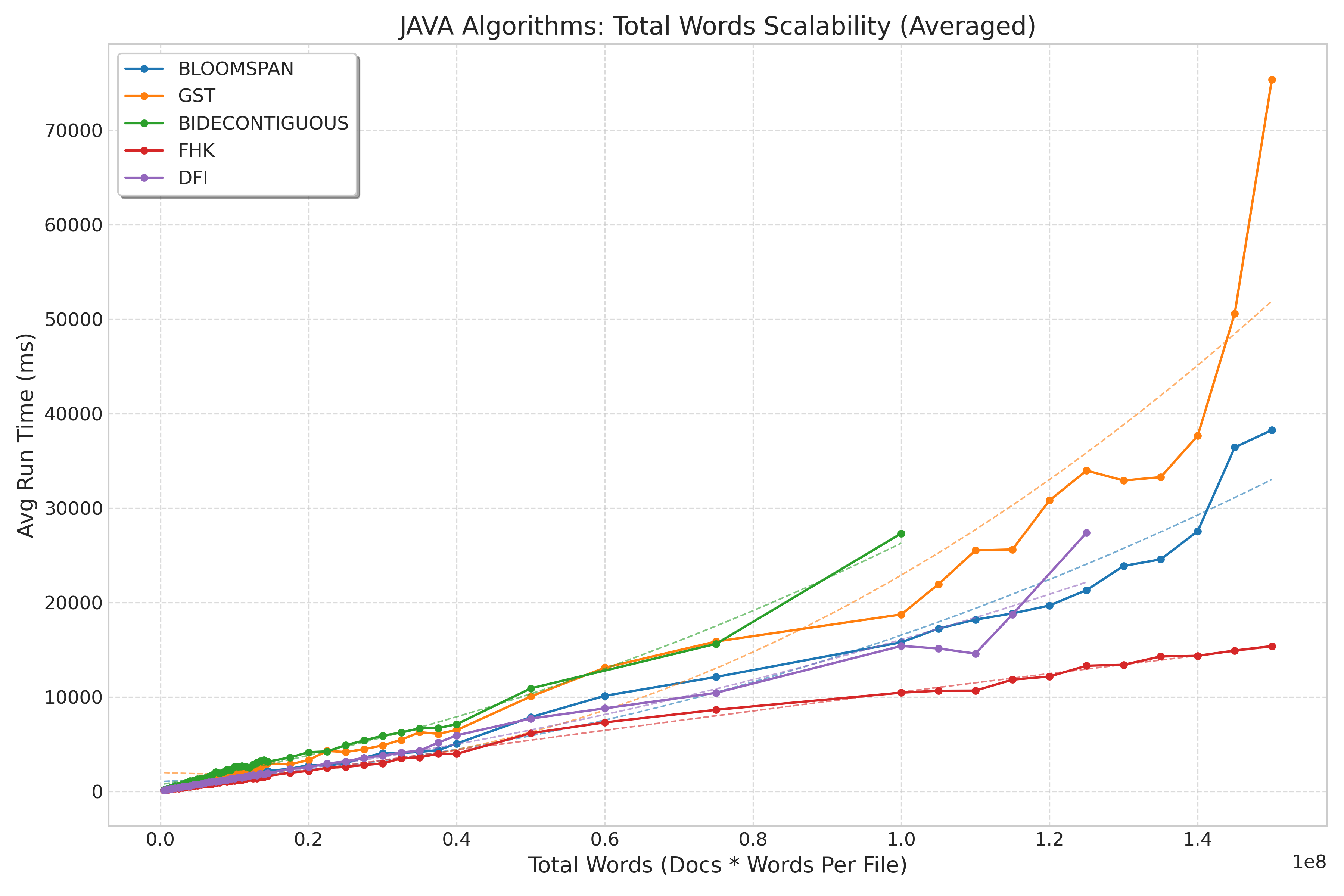
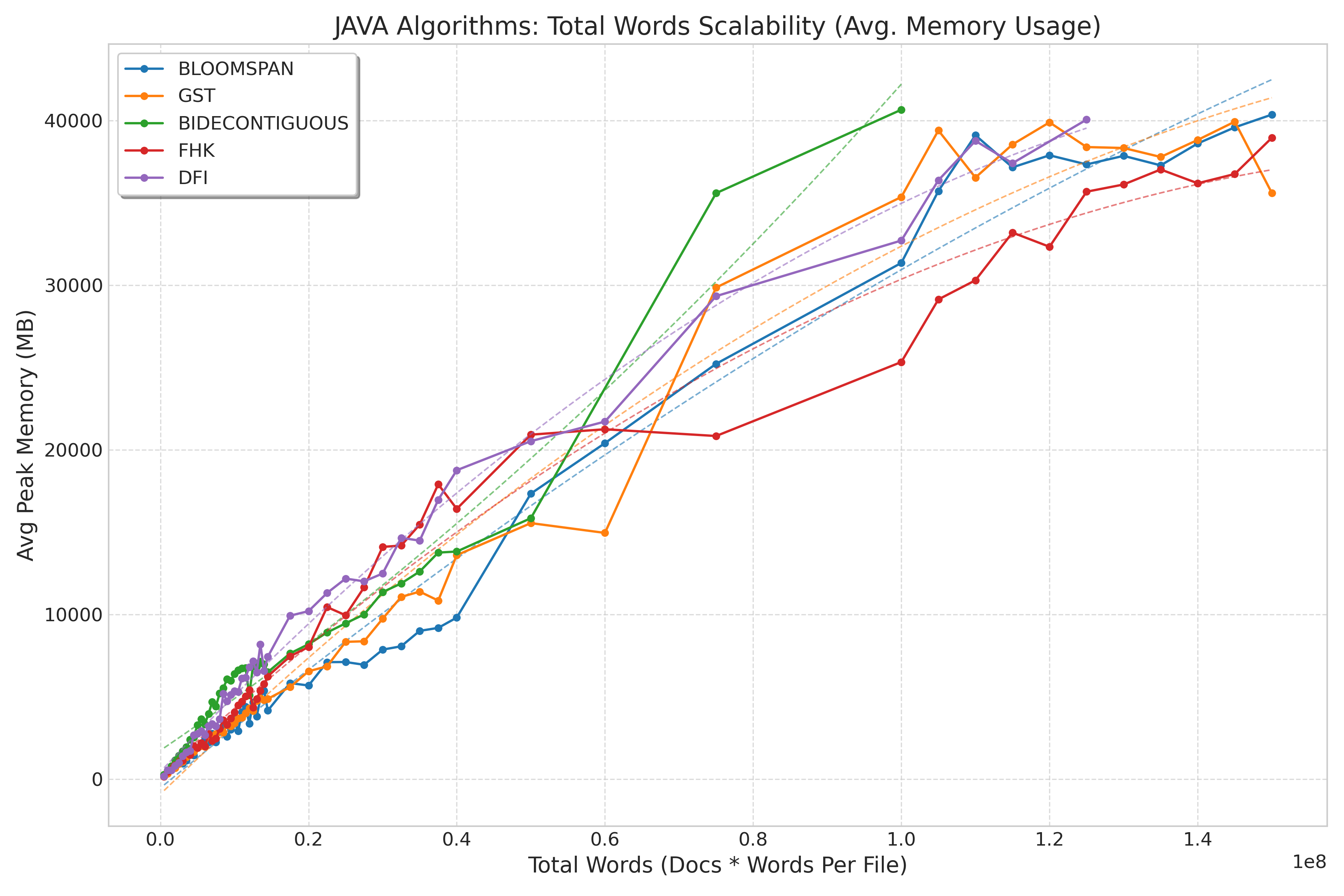
Synthetic 2 (dense nested overlaps). A deliberately constructed worst case. FHK: 10.5 s, BloomSpan: 12.6 s, DFI: 14.9 s, BIDE+ (contiguous, maximal): 16.8 s. The other SPMF algorithms: OOM.
Gutenberg-8k at a permissive threshold of σ = 10. Up to 1,000 books, BloomSpan is ≈20% faster than FHK/DFI. From 3,000 books on, FHK/DFI are 10–20% faster: at a permissive threshold, the number of frequent phrases becomes very large (≈218 thousand at 5,000 books), and again the maximality check dominates. At 8,000 books, BloomSpan runs out of memory, while FHK and DFI complete.
| books | BloomSpan, ms | FHK, ms | DFI, ms | BIDE+, ms | GST, ms |
|---|---|---|---|---|---|
| 100 | 713 | 625 | 655 | 1,275 | 2,373 |
| 500 | 3,201 | 3,896 | 4,016 | 13,241 | 27,170 |
| 1,000 | 6,608 | 8,425 | 8,313 | OOM | OOM |
| 3,000 | 28,550 | 25,427 | 25,185 | OOM | OOM |
| 5,000 | 141,023 | 117,228 | 111,864 | OOM | OOM |
| 8,000 | OOM | 2,214,653 | 1,461,332 | OOM | OOM |
Why: the "shape" of the corpus
The difference is explained not by size but by the structure of the data. A
convenient measure is the number of phrases in the Lempel–Ziv parsing divided by the number of tokens (c/n): roughly speaking,
how much the text "compresses" thanks to repeats.
- Synthetic 1: a background of unique words,
c/n ≈ 1: every background token is new, so every LZ phrase consists of a single token (an LZ78 parse of a generated corpus of 1,000 documents gives 0.99999). The background has no repeats at all: by construction, every "word" occurs exactly once. In the entire corpus, only the three inserted phrases repeat, a few dozen tokens out of tens or hundreds of millions. The distribution is flat. The Bloom filter cuts away the background, but FHK handles it just as well, and without a separate filter pass, so here the filter is pure overhead. - Synthetic 2: almost every n-gram from the inserted family is frequent. The filter has nothing to cut; all the work is in the maximality check. And FHK's LCP intervals naturally "collapse" nested overlaps.
- Natural language (Gutenberg):
c/n ≈ 0.27, about 7.94 bits per token. A Zipfian tail of rare n-grams, which the filter cuts by 98%, and a moderate number of repeats that are not pathologically nested. This is the shape of data BloomSpan was designed for. A web corpus after crawling is also natural text, just with more template repeats; by this measure, one would expect it to be closer to Gutenberg than to either synthetic set (I did not measurec/nfor a web corpus in these experiments myself).
Rule of thumb: a strict threshold and a large corpus of natural text: BloomSpan. A permissive threshold, lots of output, or data with dense nested repeats: suffix-based methods.
Part 6. Back to the index
From a list of phrases to the answer "how much junk"
A list of maximal phrases answers the question "what repeats." But the original question was "how much."
This is where the coverage mask from Part 4 comes in handy. After the algorithm finishes, it marks exactly those corpus positions that belong to at least one occurrence of some found phrase. Therefore:
- the share of marked positions in the whole corpus is the share of the index's text that consists of repeated fragments;
- the share of marked positions in each document is how "cluttered" that particular document is. The distribution of this value across documents immediately shows whether the index has pages that consist almost entirely of template (candidates for removal), and which sites or sections are more cluttered than others;
- sorting phrases by
|P| × df(P)gives the list of the "biggest index hogs": which specific fragment takes up the most tokens.
In other words, the same structure that speeds up the algorithm becomes the main metric once it finishes.
How to choose σ and the minimum length
The two parameters work like two knobs.
- σ controls "how widespread." Too low, and the answer picks up any coincidences: quotes, set expressions, identical specs of two similar products. Plus, as the tables above show, the size of the answer grows and speed drops. Too high, and templates of small sites are missed. It makes sense to start with a threshold tied to the size of a typical site in the corpus, not to the size of the corpus.
- Minimum length cuts off set phrases. A 3–4-word phrase with high support is more often language than template. Disclaimers and footers are usually longer than 10 tokens.
What to watch out for
Exact matching is a limitation. A template with a variable part ("Showing 1–20 of 345 products," "© 2019," "© 2024," the author's name in a byline) breaks into several phrases between the variable insertions. Each of them will be found individually, but as pieces rather than as one template. Support for "nearly matching" phrases (with an edit-distance tolerance) is the next step, which BloomSpan does not have yet.
Repeated does not always mean junk. In e-commerce, the same description often appears on every color and size of the same product. In news, a quote from an official statement appears in every story on the topic. In legislation, boilerplate wording is the content. The algorithm finds repeats; deciding which of them are noise is a domain decision, and you have to make it by looking at the top of the list.
Tokenization loses punctuation and case. For finding templates, this is more of a plus (minor formatting differences do not prevent a match), but it needs to be taken into account when mapping a found phrase back to the original text.
Summary
The task "find all long fragments that repeat verbatim across many documents" looks like a hash table exercise. On billions of tokens, it turns into a choice between three bad options: a hash table of n-grams does not fit in memory, sequential pattern mining algorithms drown in the combinatorics of gaps, and exact suffix-based methods build expensive structures for every token of the corpus, even for the 98% where no frequent phrase begins.
BloomSpan relies on the fact that natural text follows Zipf's law:
- a counting Bloom filter cuts away the overwhelming majority of candidates in a single linear pass and, because it only errs upward, never loses a frequent phrase;
- prioritizing by Ψ = |P| × df(P) makes the most massive templates get found first;
- depth-first growth directly on the corpus does without projected databases;
- early pruning by the left neighbor, an inverted index on the rarest token, and the coverage mask eliminate duplicate work.
On 3 billion tokens, this is 11–15 times faster than FHK, uses half the memory, and completes where the others do not fit in 40 GB. At permissive thresholds and on synthetic data with dense repeats, it loses to suffix-based methods, and that is worth knowing in advance.
And for the original task, the main thing is not even speed: after the algorithm runs, the coverage mask gives exactly the answer all of this was for: what share of the index consists of repeated fragments, and where exactly they are.
Discussion
Powered by GitHub Discussions — sign in with a GitHub account to join the conversation.