
When an online store grows to several warehouses and dozens of stores, choosing the ship-from location for each order (order sourcing) stops being a trivial task. Ship from the nearest warehouse, and you quickly burn through its capacity and stock. Ship from the one with the cheapest rate, and you create a backlog at picking that lasts for days. Assemble the order from two locations, and you pay for delivery twice and annoy the customer.
Testing a new routing algorithm on a live business is hard and expensive: today it rained, tomorrow a sale started, the day after a supplier held up a truck, and now nobody can tell why costs went up. To test algorithms under controlled conditions, I wrote osbench, a discrete-event simulator of a fulfillment network.
Inside the simulator, virtual time flows with one-minute precision. Shoppers in different cities fill their carts, the storefront promises them a delivery date, anti-fraud checks their cards, the order management system (OMS) looks for a warehouse, warehouse workers come in for their shifts and pack boxes in waves, carriers pick up pallets on schedule, and the purchasing department restocks the shelves.
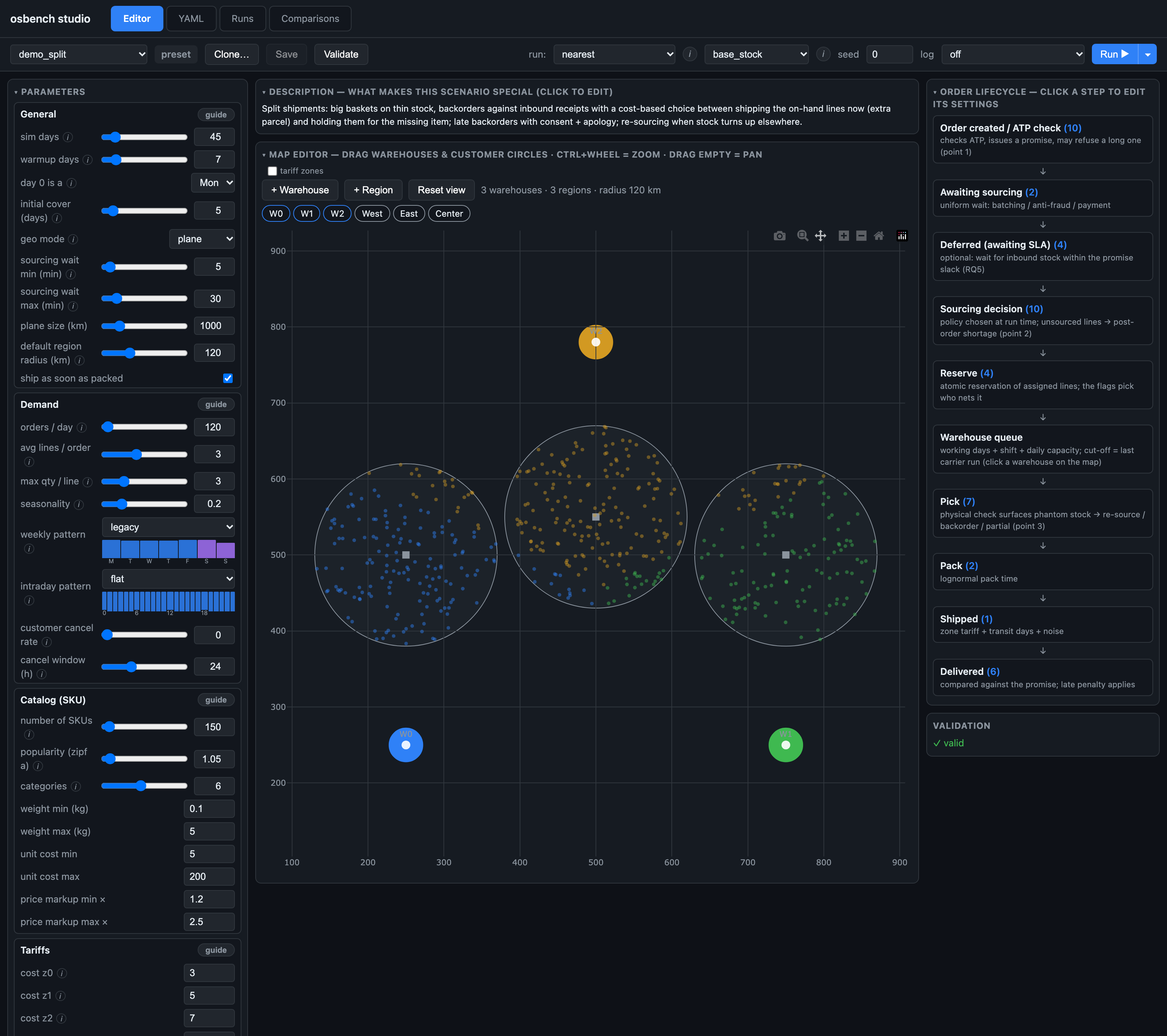
osbench studio scenario editor. Parameters by section on the left, the scenario description and the map in the center, the order lifecycle diagram on the right. At the top: policy selection, the seed, and the run button.How an experiment works and why it all comes down to money
At the core of the engine is an event queue: "order created," "payment check finished," "pick wave formed," "shipment arrived." The rules of this world are defined entirely in a YAML config or through the osbench studio visual interface.
The simulator's key feature is deterministic handling of randomness. The master seed is split into independent random number generators: separate ones for geography, the catalog, order arrivals, lead times, picking speed, accounting errors, and customer behavior. Every random event is tied to the key of a specific entity. If two different warehouse selection algorithms run on the same seed, they see the same shoppers with the same carts at the same minutes. Even if one algorithm sent an order to Kazan and the other to Moscow, the customer's reaction to a late delivery or the supplier's delay on day 14 will be identical. Any difference in the final numbers is explained by the algorithm's decisions.
Comparing algorithms on a single operational metric is awkward: one delivers fast and expensively, another saves on shipping at the cost of cancellations and late deliveries. So the simulator converts every event into money and rolls everything up into a single figure: the average cost per order, total_cost_per_order.
osbench run --scenario small --sourcing nearest
After a run, the working folder contains an event log, daily inventory snapshots, and a metrics.json file. The total cost per order is the sum of operating costs and penalties for lost service level:
| Component | Economic meaning |
|---|---|
shipping_cost |
carrier rate + picking and packing at the warehouse (per line item and per box) |
holding_cost |
storage cost: physical stock on the shelf × daily rate |
purchase_cost |
buying goods from the supplier |
penalty_cost |
penalties for lost sales: rejection at checkout, cancellation of an accepted order, shortage at picking |
lateness_penalty_cost |
penalty for each day of delay past the date promised to the customer |
| Other items | inter-warehouse transfers, surcharge for splitting an order into several boxes, apology coupons, cycle counts, return processing |
The first two weeks of a run (warmup_days: 14) don't count. At the start of the simulation, the warehouses are filled with initial stock, the picking queues are empty, and the system needs time to settle into its working rhythm.
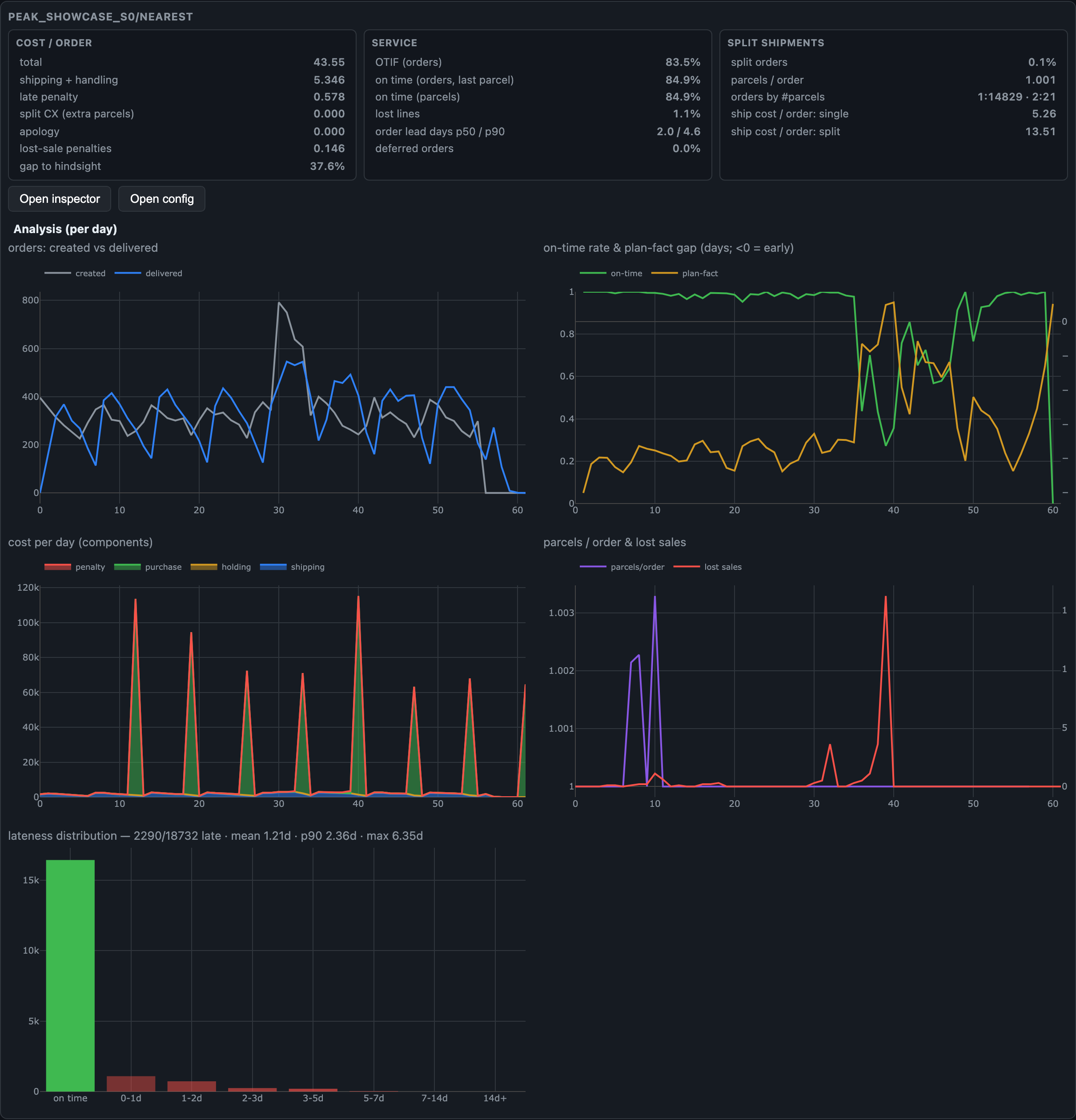
demo_calendar run on the Runs tab: orders created and delivered, on-time share and the "plan vs. actual" gap, costs by component, parcels per order and losses, the lateness distribution. The "Open inspector" button opens the same run in osbench replay.Geography, catalog, and demand
Before sending orders down the pipes, the simulator builds the world: it places cities and warehouses, makes deals with carriers, and fills the catalog with products.
Cities, warehouses, and rate zones
The map can be flat, in kilometers (plane), for synthetic tests, or spherical, with real latitude and longitude coordinates (haversine). Shoppers live in regions around city centers. The population_weight parameter sets the city's share of total demand, and radius_km sets the radius within which customers live.
geo: { mode: plane, plane_size: 1000.0 }
region_radius_km: 20.0
regions:
  - { region_id: 0, name: Moscow, x: 100, y: 100, population_weight: 1.0 }
  - { region_id: 1, name: Kazan,  x: 900, y: 100, population_weight: 0.5, radius_km: 60 }
warehouses:
  - { warehouse_id: 0, name: W0, x: 200, y: 200, capacity_lines_per_day: 500 }
In a compact city, all shoppers fall into the same rate zone relative to a warehouse. But if you define a wide metro area (radius_km: 60), residents of different outskirts of the same city end up in different rate zones, and the optimal warehouse differs for them. The demo_contested scenario is built on this effect. In the Studio visual editor you can drag regions and warehouses with the mouse, and the rate zone boundaries are highlighted right away.
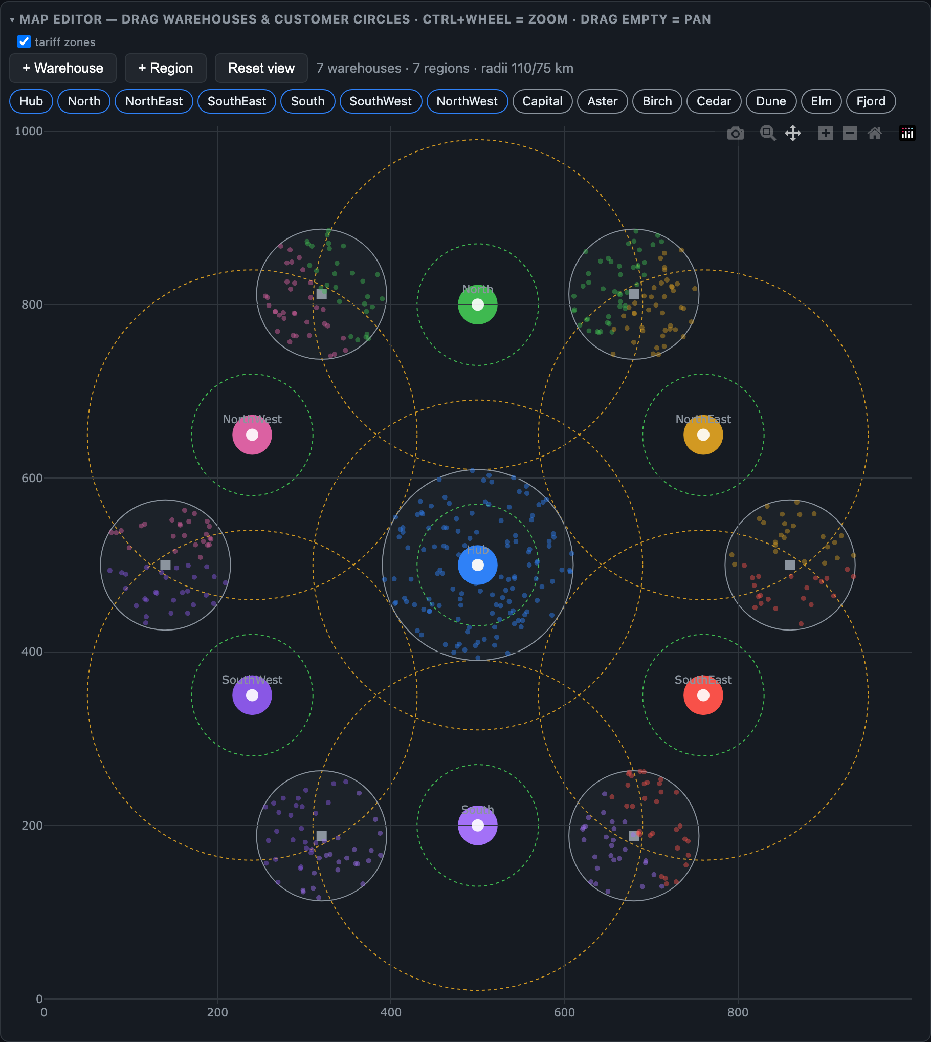
Shipping is priced on the classic zone grid used by parcel carriers: the distance from the warehouse to the customer determines the zone number, and the zone determines the base rate per box, the surcharge per kilogram of weight, and the standard transit time.
tariffs:
  zone_bounds_km:       [50, 300, 1000, 1e9]
  cost_by_zone:         [3.0, 5.0, 7.0, 10.0]   # base rate per parcel
  per_kg_by_zone:       [0.1, 0.2, 0.3, 0.5]    # surcharge per kg
  transit_days_by_zone: [1, 2, 4, 7]
  steepness: 1.0
  delivery_noise_days_mean: 0.0
A 2 kg parcel going 250 km falls into the second zone: it costs 5.0+0.2x2=5.4 units and takes two days. The steepness multiplier scales the whole rate grid at once, so you can check how the logistics will behave if freight gets 30% more expensive. The delivery_noise_days_mean parameter adds random in-transit delays (geometric distribution), turning an ideal carrier into a real one that promises two days but sometimes takes four.
The warehouse itself has a price list too: picking one line item (order line) costs handling_cost_per_line (0.5 by default), packing a box costs handling_cost_per_parcel, and storing one unit for a day costs storage_cost_per_unit_day (0.01). You can also give a warehouse a rank priority to tell your own distribution centers apart from expensive partner 3PL warehouses.
Products and Zipf's law
In a real online store, a few dozen hits bring in half the revenue, while thousands of items sell one unit a month. In the simulator, product (SKU) popularity follows a Zipf distribution with the curvature parameter zipf_a.
sku:
  n_sku: 500
  zipf_a: 1.1
  n_categories: 5
  weight_kg_range: [0.1, 5.0]
  unit_cost_range: [5.0, 200.0]
  price_markup_range: [1.2, 2.5]
With 500 products and zipf_a: 1.1, the top bestseller accounts for 19% of all unit sales, the hundredth most popular product for about 0.1%, and the tail of the catalog for hundredths of a percent. If you need to model a fierce battle for scarce hits, just raise zipf_a to 1.4 on a short catalog. Weight, purchase price, and retail markup are generated randomly within the given bounds and don't depend on the product's popularity.
By default, all cities "like" the same products. But if you set the region_category_matrix, regions get their own preferences: the north buys one category more actively, the south another, and stock of the same size at the warehouses starts draining at different rates.
Order rhythm and the calibration trap
Orders arrive as a non-homogeneous Poisson process. Each order has a random number of line items (geometric distribution with mean lines_per_order_mean: 1.6, so orders of one or two items dominate) and from 1 to qty_max units in each line.
The base order rate base_orders_per_day is multiplied by annual seasonality, a day-of-week profile, and an hour-of-day profile:
demand:
  base_orders_per_day: 200
  lines_per_order_mean: 1.6
  qty_max: 3
  seasonality_amplitude: 0.2
  weekly_profile: ecom_b2c       # peak on Monday, dip on Friday and Saturday
  intraday_profile: b2c_evening  # evening peak 19:00–22:00, quiet at night
There are ready-made profiles for the weekly and daily rhythm: classic B2C with an evening peak and a Monday spike, office purchasing strictly on weekdays from 9 to 6, weekend retail, or express delivery with two humps at lunch and in the evening. The intraday profile only redistributes orders within the day, keeping their daily count and basket contents. This lets you run a clean paired experiment: how will the share of late deliveries change if, at the same daily volume, shoppers start placing orders in the evening, after the day's truck has already left the warehouse?
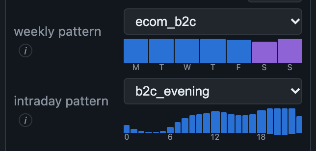
demo_calendar: the weekly profile ecom_b2c with a Monday peak and weekends marked, the intraday profile b2c_evening with an evening peak.The journey of a single order
Let's follow what happens to an order from the second the shopper clicks "Place order" to the moment the courier hands over the box. In Studio, this route has its own interactive diagram: clicking any stage opens its settings.

Storefront, availability check, and the promised date (Promise)
In the cart, the shopper sees the promised delivery date, the promise (delivery promise). How bold a promise the storefront makes affects both the purchase conversion and future penalties for late delivery. The promise is calculated from the warehouse with the fastest delivery to the customer's city, in one of four ways:
zone_fixed: the minimum warehouse processing time plus the transit time for the rate zone. The most aggressive option, with no room for error.transit_plus_buffer(the default): adds a safety margin ofbuffer_daysto the base time.atp_based: if the product isn't in the warehouse right now but a shipment is expected in 4 days, the storefront honestly adds those 4 days to the delivery time.percentile: a statistical calculation that takes a given quantile of the carrier's random delays so as to meet the promised date, for example, 90% of the time.
If you enable calendar_aware: true, the storefront checks the warehouse's working calendar when calculating the promise and won't promise to ship on a Saturday from a warehouse that's closed on weekends.
Customers don't like to wait too long. The cap_days parameter sets the maximum time the site is allowed to show at all, and p_accept_promise sets how willing the shopper is to put up with waiting. At 0.6, the probability that the customer accepts the delivery date falls linearly from 100% at the zone's base time to 60% at the cap_days limit. If the date doesn't suit them, the shopper abandons checkout, and the system records a lost sale (PROMISE_REJECTED) with a penalty_lost_sale penalty (5 units by default).
An available-stock check can also run right at checkout (checkout_atp_check: true). When it's on, the storefront checks whether at least one warehouse in the network can ship each line of the cart in full. If some product is short, the shopper accepts a substitute from the same category with probability p_substitute, buys a trimmed cart without the scarce item with probability p_partial, and otherwise abandons the order altogether. If the checkout check is off (the default behavior), the site optimistically accepts any order and shifts the headache of shortages onto the OMS and the warehouse.
Order intake: address, payment, and anti-fraud checks
A placed order doesn't reach the warehouse in the same second. First it goes through a pipeline of checks (intake): address validation, payment processing, and fraud monitoring.
intake:
  address: { auto_minutes: [0, 1], p_hold: 0.02, hold_hours_mean: 6,
             hold_window: [540, 1260], p_reject_after_hold: 0.3 }
  payment: { auto_minutes: [0, 2], p_reject: 0.01, p_hold: 0.03, hold_hours_mean: 0.5,
             p_reject_after_hold: 0.4, reject_cost: 5.0 }
  fraud:   { auto_minutes: [0, 1], p_reject: 0.002, p_hold: 0.02, hold_hours_mean: 3,
             hold_window: [540, 1080], p_reject_after_hold: 0.2 }
  reserve_during_checks: false
Each step has two-loop logic. The fast automatic loop takes a couple of minutes (auto_minutes) and immediately weeds out obvious junk with probability p_reject (a nonexistent address, a bank decline, a triggered anti-fraud block rule). Suspicious orders go to manual review with probability p_hold: call center agents confirm the address, the customer goes through 3-DS again, and fraud analysts study the shopper's profile.
Manual review takes hold_hours_mean hours on average, but the timer only ticks during the relevant team's working hours (hold_window, in minutes from midnight). If an order lands in manual anti-fraud review at 11 p.m. and the analysts work from 9:00 to 18:00 ([540, 1080]), it sits untouched until morning. Orders rejected at this stage (ORDER_REJECTED) don't spoil the lost-sales and on-time delivery statistics (OTIF, On-Time In-Full), since it was the store that walked away from the deal, but each rejection costs the company reject_cost (agents' work, fees, lost profit).
I should point out right away that the simulation doesn't include the call center or the delivery, because each of these areas deserves a full-fledged simulator of its own and adds a lot of complexity without adding anything useful to the simulation experiments. In other words, the call center is assumed to have unlimited capacity and delivery to be 100% reliable (both assumptions have little to do with reality). But when the main goal revolves around warehouse selection algorithms, what happens with delivery, for example, doesn't really matter much.
So, moving on. Here we hit an important architectural fork, controlled by the reserve_during_checks flag: at what point do you choose the warehouse and reserve the goods?
- With
false, the order looks for a warehouse only after it has passed all the checks. While a nighttime order waits for the morning fraud analyst, other customers may buy up the last units in the warehouse. - With
true, the OMS chooses the warehouse and places the reservation instantly at checkout, but doesn't allow the pick task to be passed to the warehouse management system (WMS) until anti-fraud gives the green light. This protects an honest shopper from losing the goods, but freezes stock under fraudulent and unpaid orders.
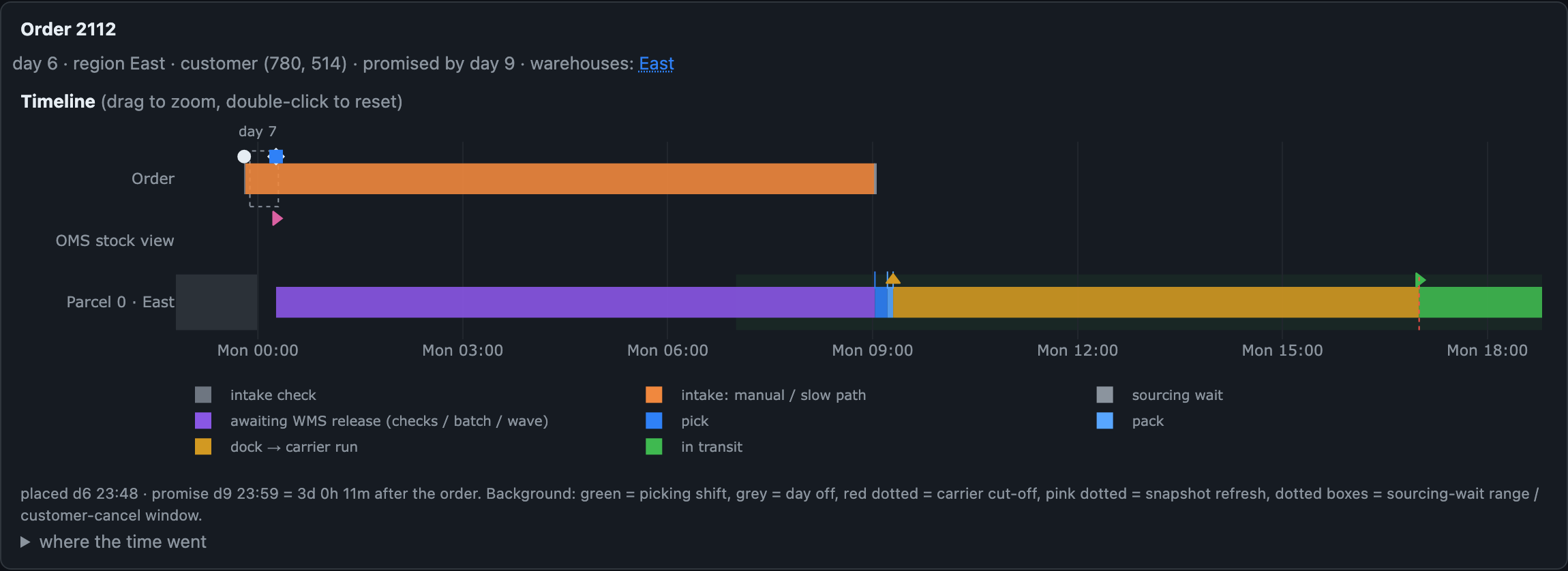
hold_window: [540, 1080]), reserve_during_checks: true. The order came in at night and went to manual review (the orange segment in the "Order" lane), which stays put until the window opens at 09:00. The warehouse is chosen and the goods are reserved almost immediately, but the parcel waits all night to be handed off to the WMS (the purple segment) and goes to picking only after approval.Even after all the checks, the order spends between 5 and 30 minutes in the OMS's own buffer (sourcing_wait_min..max); this models batch processing of the sourcing queue. Meanwhile, the shopper's own timer is ticking: with probability cancel_rate, the customer may change their mind and cancel the order within the first cancel_within_hours hours, before picking has started at the warehouse.
Inside the warehouse: schedule, waves, picker pace, and cut-off
Once the OMS has chosen the warehouse and reserved the goods, the task needs to be passed to the warehouse management system (WMS) and picked by hand.
Real warehouses rarely start running down the aisles for each individual purchase the second it comes in. The handoff of tasks from the OMS to the WMS is configured with the release_mode parameter:
immediate: one-by-one handoff right after the reservation;periodic: a batch release on a schedule everyrelease_period_minminutes;waves: release in waves at fixed hours on working days (wave_times_min: [480, 660, 840, 1020]corresponds to waves at 08:00, 11:00, 14:00, and 17:00), timed to the carrier's truck arrivals.
The warehouse itself runs on a working schedule: the working days of the week (work_days: no days off, a six-day week, or weekdays mon-fri) and the shift hours (shift_start_min and shift_end_min). Warehouse capacity is limited by two ceilings: the daily limit capacity_lines_per_day and the hourly throughput of the picking crew pick_lines_per_hour.
warehouses:
  - { warehouse_id: 0, ..., work_days: mon-fri, shift_start_min: 480, shift_end_min: 1200,
      cutoff_min: 960, release_mode: waves, wave_times_min: [480, 660, 840, 1020],
      pick_lines_per_hour: 120 }
When the crew's hourly pace is set, orders don't all pile into picking at once at the start of the shift; instead, they join a live queue for the pickers. When a parcel's turn comes, the actual walk through the warehouse with a scanner (pick) and packing into a carton (pack) take a random time drawn from a lognormal distribution:
process_times: { pick_median_min: 10, pick_per_line_min: 3, pack_median_min: 5, sigma: 0.3 }
At the median, a picker spends 10 minutes on the approach and 3 minutes on each line item, and another 5 minutes go to packing. Anything the crew didn't get to before the end of the shift or beyond the daily limit stays put until the next working morning.
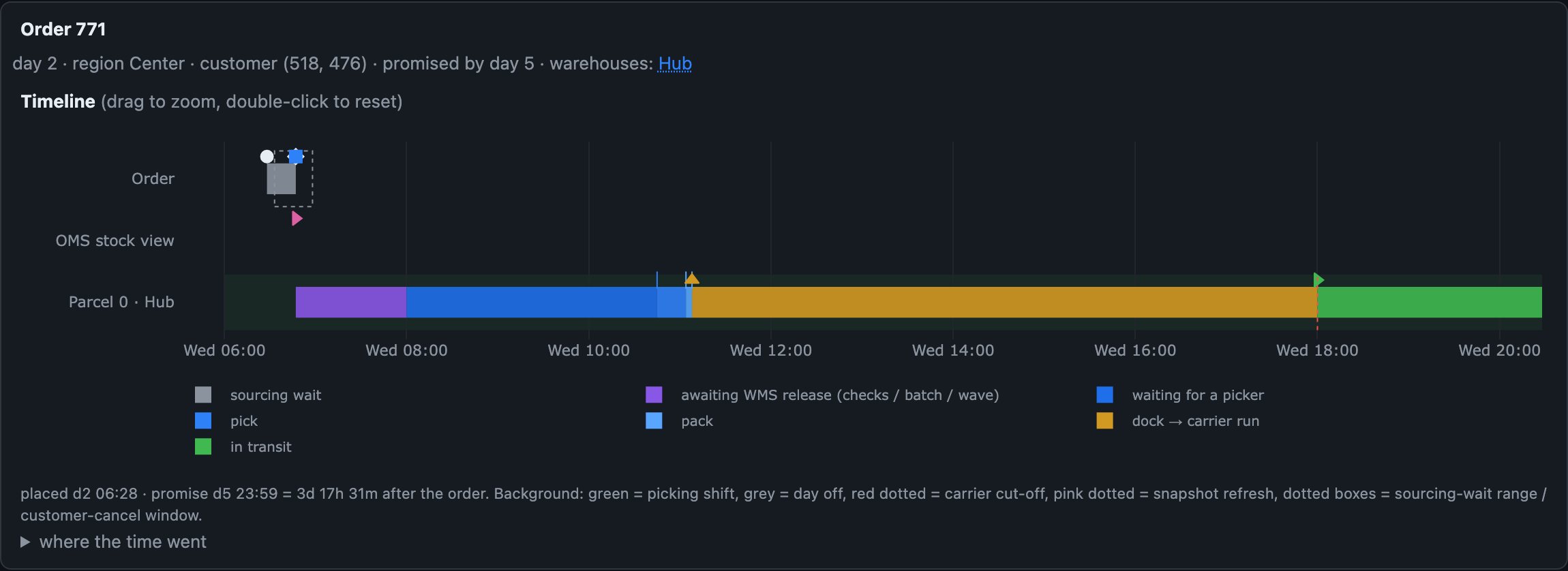
The packed box goes to the shipping dock and waits for the carrier's truck. Each warehouse has a cut-off time, the cut-off (cutoff_min, 16:00 by default). Boxes packed before 16:00 leave on the evening run (if the truck had room within the daily carrier_parcels_per_day quota). A box taped up at 16:05 stays on the dock overnight until the next working day. If this happened on a Friday at a warehouse with a five-day work week, the parcel won't leave until Monday evening.
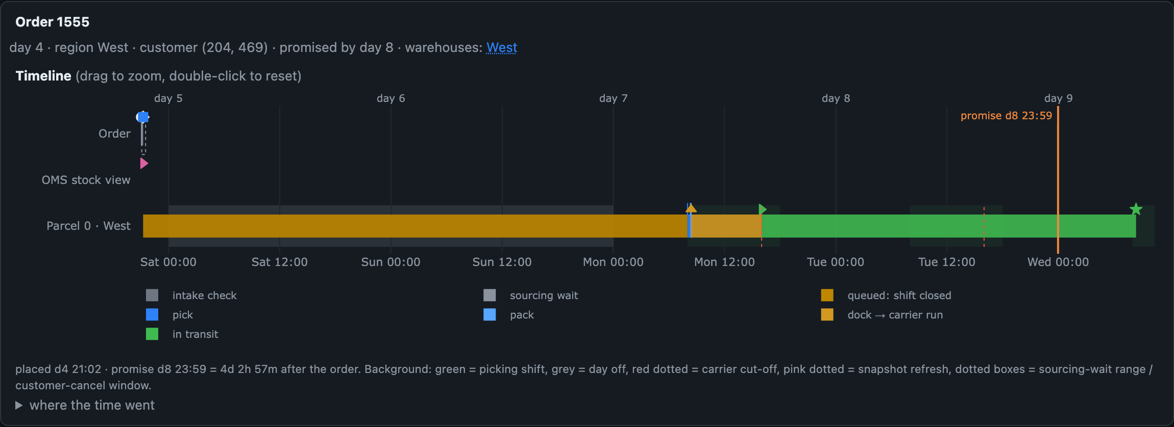
osbench replay. The order was placed on Friday evening and assigned to the West warehouse (Mon–Fri). Green background is the picking shift, gray is the weekend, the red dashed line is the carrier cut-off, the orange vertical line is the promise. The parcel sits in the "shift closed" queue all weekend, is picked on Monday at 08:00, and goes to the carrier at 16:00.By default, late deliveries carry no monetary penalty. But as soon as we enable penalty_late_per_day: 4.0 in the config (a penalty for each day of delay, charged either to the whole order based on its slowest parcel or to each late line), warehouse overload and missed cut-offs start bankrupting the company fast.
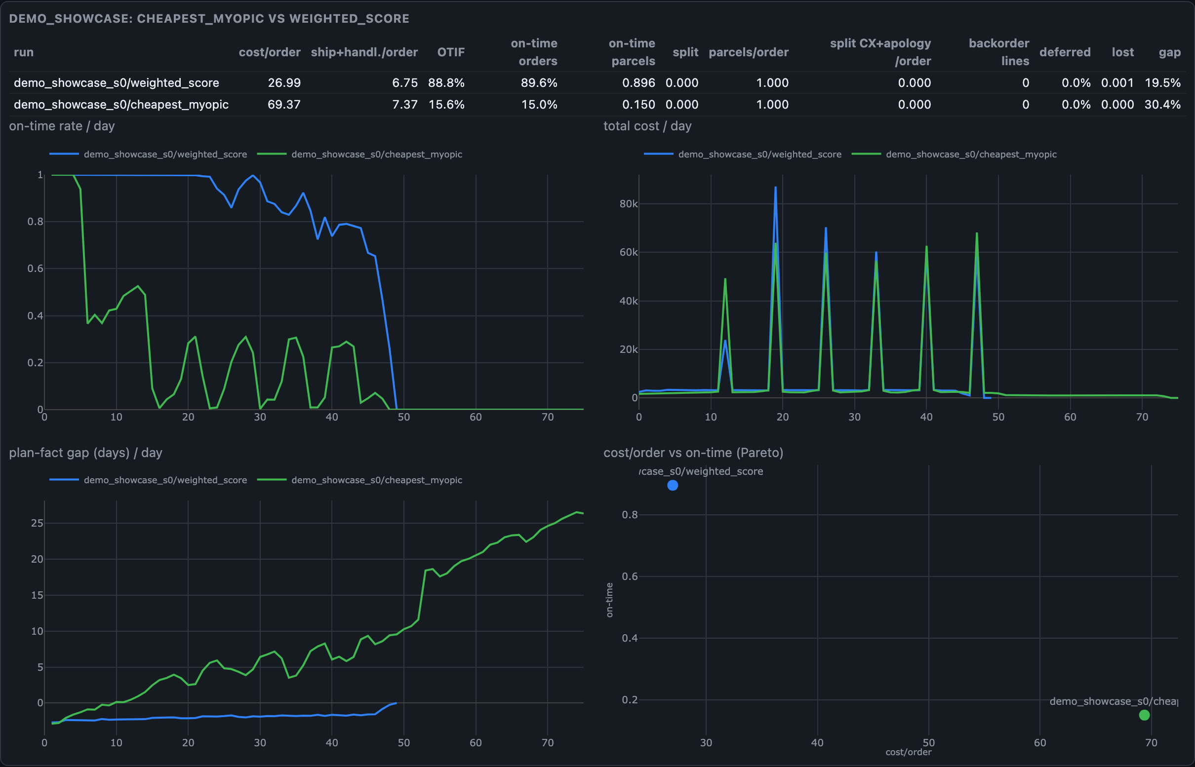
cheapest_myopic and weighted_score on the same demo_showcase seed with a lateness penalty. weighted_score costs 27.0 per order with 89% of orders on time, cheapest_myopic costs 69.4 with 15%. The greedy policy overloads one warehouse, its "plan vs. actual" gap keeps growing throughout the run, and almost all of the cost difference comes from lateness penalties.Inventory, replenishment, and shadow lost units
For a warehouse to ship anything, the goods have to be on the shelf. But in real life there's almost always a gap between what is physically on the shelf and what the sourcing algorithm sees in the database.
Four views of stock and the ATP formula
For each product at each warehouse, the simulator keeps five counters in parallel:
phys: how many units are physically on the rack right now;book: the book stock in the warehouse management system (WMS) database;reserved: how many units are already promised to accepted orders but not yet taken off the shelf by pickers;in_transit: goods on their way from a supplier or from another warehouse;safety: an untouchable safety stock that may not be spent on online orders.
The quantity that can be freely promised to a new shopper is called ATP (Available to Promise). Depending on the company's settings, ATP is calculated in different ways:
on_hand_only: book minus reserved (we sell everything down to the last unit on the books);basic(the default): book minus reserved minus safety (we keep a safety cushion);cumulative: adds tobasicthe future receipts (in_transit) due at the warehouse within the nexthorizon_daysdays. The future receipt may only be shown to the storefront (for the availability check and the delivery date calculation), while the warehouse selection at fulfillment works with on-handbasicstock or puts the order on a waitlist for the shipment.
Assortment matrix, stock levels, and purchasing
Warehouses rarely carry the entire catalog. The assortment_fraction: 0.6 parameter means that a given warehouse carries a random sample of 60% of the products (the generator makes sure that each product is sold from at least one warehouse in the network). It's this partial assortment overlap that most often forces the system to split a multi-item order across warehouses.
At the start of a run, the engine estimates the average daily demand for each product and calculates four norms for each "product–warehouse" pair:
- Initial stock = (demand per day) x (
initial_cover_days), which is also trimmed if the warehouse hits its total rack capacitystorage_capacity_units; - Safety stock (
safety) = (demand per day) x (safety_days); - Reorder point (
s) = (demand per day) x (average lead time); - Order-up-to level (
S) = (demand per day) x (lead time + review period) x (S_overshoot).
Let's see what numbers come out in the small preset (4 warehouses, 14 days of stock, a purchasing review every 7 days, a supply wait of ~4.3 days):
| Catalog position | Demand per warehouse per day | Initial stock | Safety stock (safety) |
Reorder point (s) |
Upper level (S) |
|---|---|---|---|---|---|
| Top hit (rank 1) | 30.7 units | 430 units | 15 units | 133 units | 522 units |
| Mid-range item (rank 100) | 0.19 units | 3 units | 0 units | 1 unit | 4 units |
| Long tail (rank 500) | 0.03 units | 1 unit | 0 units | 1 unit | 1 unit |
The last row neatly explains the nature of stockouts in e-commerce: a rare product sits in the warehouse as a single unit. If two orders for it come in during the same week, the second one will inevitably run into a stockout.
Every review_days days, the purchasing module checks the current inventory position (book + in_transit - reserved) and sends orders to the supplier with lead time lead_time_days (with a lognormal spread of lead_time_std_days), rounded up to the minimum order quantity moq, which gives the stock chart its characteristic sawtooth shape.
The simulator implements six replenishment policies (--replenishment): the classic base_stock (order up to S every cycle), s_S (order up to S when stock drops below s), and R_Q (order in multiples of pallets of Q units); the adaptive forecast_driven (recalculates S from actual sales with a service factor); the centralized network_allocation (buys for the whole network and divides the shipment in proportion to the warehouses' actual shipments); and a special scheduled mode that turns off the feedback loop and strictly replays a prerecorded receipt schedule.
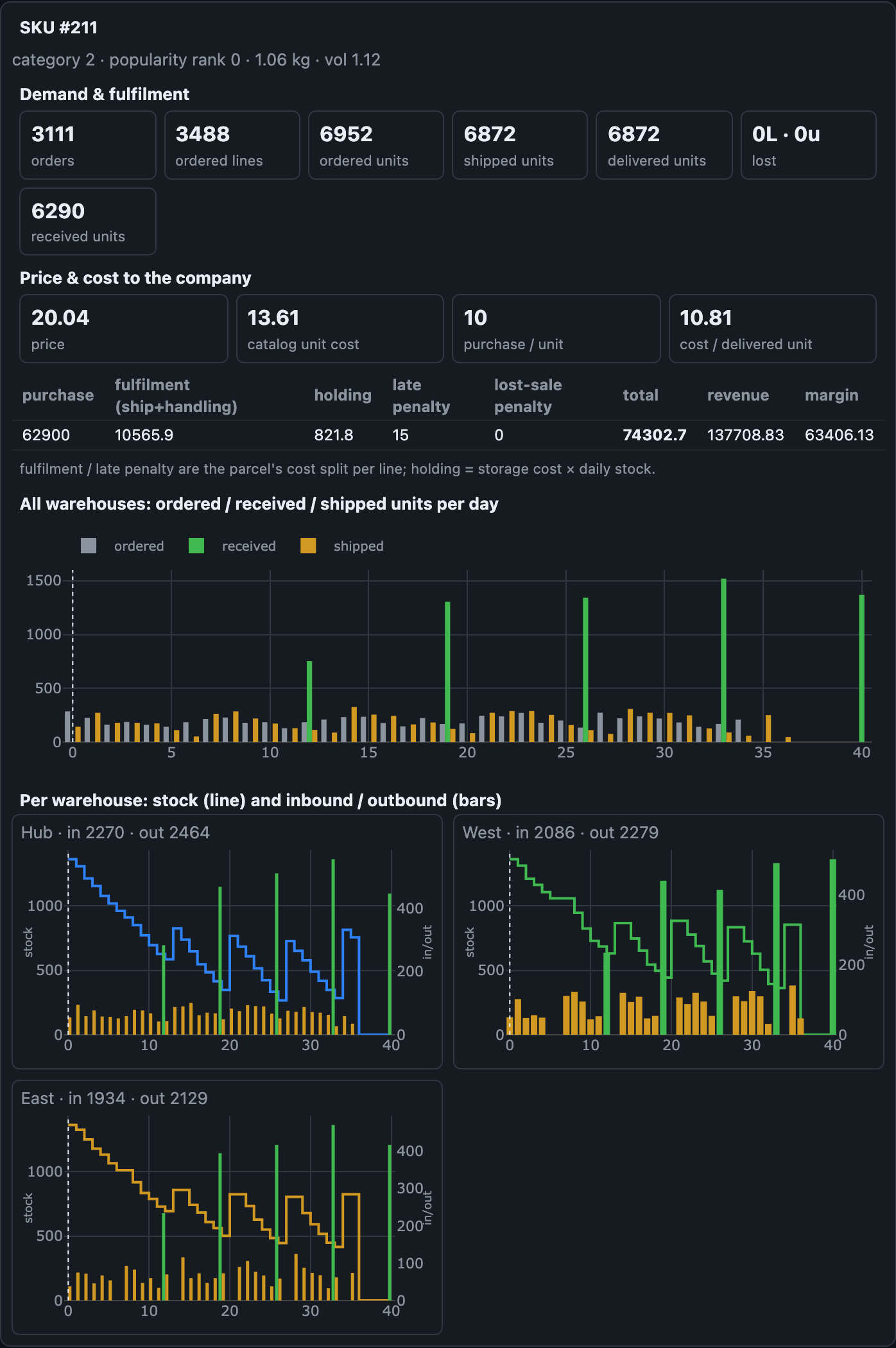
demo_calendar. At the top: ordered, received, and shipped across the whole network per day. Below, for each warehouse: the line is stock, the bars are receipts and shipments. Stock is used up and replenished once per review cycle, hence the "sawtooth."How stockouts happen and where phantom stock comes from
A shortage can surface at one of three stages, and the later it happens, the harder it hits the reputation and the wallet:
- At checkout (
penalty_lost_sale: 5): an honest "out of stock" before payment. - In the OMS after the order is accepted (
penalty_post_order: 8): the money has been charged and the order accepted, but during sourcing no warehouse within the allowed times and rates (atp.tolerance_*) could cover the line, and calling the customer to offer a longer wait (p_accept_slow) didn't help. - At picking (
penalty_pick: 10): the nastiest failure: the OMS was sure the product was there, sent the task to the warehouse, the picker walked up to the bin, and the shelf was empty.
Why was the product on the books (book > 0) but not on the shelf (phys == 0)? In the simulator, a shortage at picking has four physical causes, which are tracked separately in the shortage_pick_causes metric:
- Receiving error and phantom stock (
accounting_error). With each truck unloading, with probability1 − inventory_accuracy.accuracy(for example, in 3% of shipments), the receivers make a mistake and put on the shelf, on average,error_meanfewer units than they post in the WMS. This "phantom stock" lingers in the database until a picker comes for the last unit and finds an empty bin. You can fight phantoms before a customer order runs into them with regular cycle counting (cycle_count_days: 14,cycle_count_cost_per_location: 0.2): every day, auditors walk 1/14 of the racks and reconcile the book numbers with the shelf. - No reservation (
no_reservation_conflict). Two orders claimed the last unit of a product at the same time because the OMS didn't place a hold. - Stale stock snapshot (
stale_snapshot). The warehouse has already written the product off, but the integration bus hasn't delivered the news to the OMS yet. - Snatched on the sales floor (
walkin_conflict). When shipping from a retail store, an ordinary walk-in shopper managed to grab the last unit off the display and pay for it at the register while the online order picker was walking to the shelf.
If a picker runs into an empty shelf, the OMS tries to save the order: it moves the line to another warehouse that physically has the product (p_resource), puts the line on hold until the nearest shipment (backorder), or cancels the line for good with the maximum penalty.
Warehouse selection algorithms and handling splits
Once an order has passed the checks and reached sourcing, the OMS builds a list of candidate warehouses where the product is in the assortment and in stock. Twelve built-in policies (--sourcing) solve the problem of choosing the ship-from location:
Algorithm (--sourcing) |
How it works | Where it's used in practice |
|---|---|---|
random |
a random warehouse that has the product | a lower bound for sanity checks |
nearest |
the warehouse nearest the customer that can fulfill the whole order; otherwise, the fewest boxes | the basic rule of most off-the-shelf OMSs |
cheapest_myopic |
tries combinations of warehouses and minimizes the sum of shipping, picking, and the split penalty right now | greedy logistics optimizers that ignore load and tomorrow's demand |
weighted_score |
computes a weighted score from 7 normalized factors | industrial OMSs (SAP Commerce, Adobe Commerce, etc.) |
weighted_score_tuned |
the same formula, but the weights are fitted by an optimization algorithm (osbench tune) on historical runs |
scoring calibrated for a specific network |
spillover_limit |
picks the cheapest warehouse but forbids spending more than X% of the warehouse's daily capacity on orders from other regions | protecting regional warehouses from being overloaded by neighbors |
primal_dual |
adds to the shipping rate a dynamic shadow price of the product that rises as the shelf empties | online protection of scarce stock without building forecasts |
dtlp_bidprice |
periodically solves a linear programming (LP) problem on a demand forecast; the dual values serve as the opportunity cost of giving stock to another region | the classic academic algorithm by Acimovic & Graves (2015) |
rolling_milp |
regularly recalculates optimal "region → warehouse" flow quotas, taking warehouse capacity into account | rolling volume and calendar planning |
hindsight_lp |
a global optimization that knows all future orders until the end of the run in advance | an ideal unreachable in real life (an upper bound on the network's potential) |
wait_or_split |
weighs three alternatives in money: split the order now, create a backorder, or freeze the order until the shipment arrives | advanced consolidation of multi-line orders |
The industry standard weighted_score rates each candidate on seven criteria (normalizing them from 0 to 1 among the warehouses available for this order): distance to the customer (weight 0.20), shipping cost (0.20), time slack before the promised date (0.25), ability to ship the whole cart as one parcel (0.10), stock depth above the safety level (0.10), today's capacity utilization of the warehouse (0.10), and the warehouse's rank priority (0.05).
Order splits, backorders, and waiting for a shipment
What should you do if a shopper ordered four items, three of which are at warehouse A, and the fourth isn't anywhere (but a truck with it will arrive at warehouse B in three days)?
If you simply split the order into two parcels from different warehouses, the company pays three times: for a second carrier base rate, for packing a second box (handling_cost_per_parcel), and for the annoyance of a customer who has to meet two couriers (cx_penalty_per_extra_parcel: 1.5). And if the returns module is on, there's a fourth blow: customers who received their order in parts return their purchases returns.split_uplift more often.
Instead of splitting right away or canceling, the simulator lets you use two time-based mechanisms: backorder and deferral.
With backorder enabled (shortage.backorder: true), the scarce fourth line is firmly reserved against a specific upcoming shipment to warehouse B. The fate of the first three lines, which are already at warehouse A, is decided by the backorder_shipment setting:
ship_available: the three in-stock items go to the customer right away, and the fourth catches up with them as a second parcel after the truck is unloaded;consolidate: the system holds the whole order and ships all four items in one box after the goods arrive;cost_based: a calculator inside the OMS computes the cost of both options (an extra box and the split penalty vs. the risk of the whole order being late and having to give the customer an apology coupon,apology_cost: 3.0) and picks whichever is cheaper for the business.
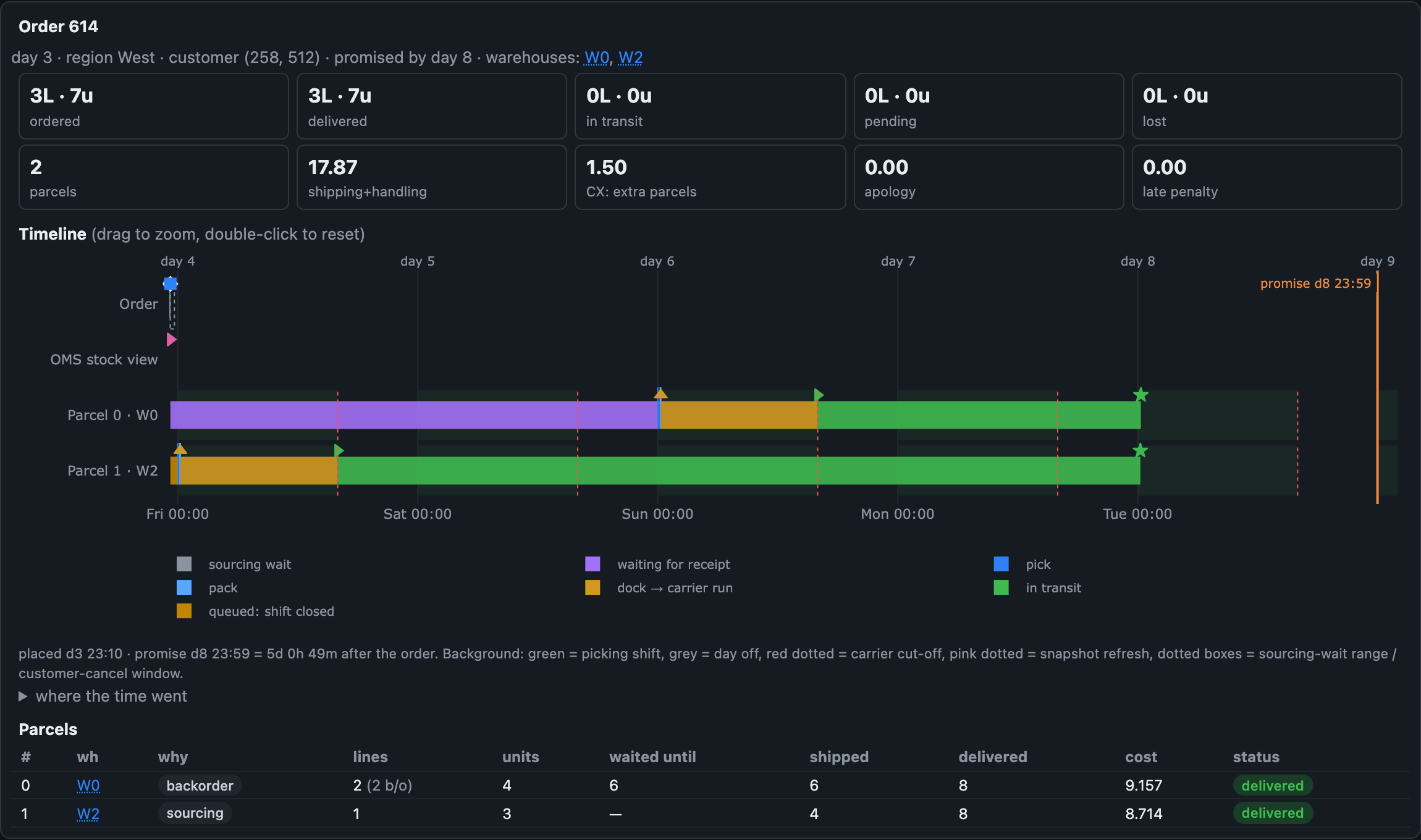
demo_split. The lines that were in stock were picked at one warehouse and left right away. The missing line at another warehouse waited about two days for a shipment (the purple "waiting for receipt" segment) and left as a separate parcel. In the parcels table its reason is backorder, and the summary shows the cost of the second box ("CX: extra parcels").Deferral (deferral.mode: wait_for_receipt or wait_to_consolidate) works differently: the OMS doesn't choose a warehouse or place any reservations at all, but parks the order in a waiting buffer until a calculated deadline (set so that after the shipment arrives there's still time to pick the parcel and deliver it by the promise). As soon as a shipment with the needed product arrives at any warehouse, the waiting orders wake up and line up according to an arbitration rule (edf: whoever's promise deadline is closest; fifo: whoever has waited longest; value: whoever's order is worth more). Unlike a backorder, a deferred order doesn't tie other shoppers' hands with a firm hold, but it risks ending up with nothing if higher-priority neighbors in the line snap up the arriving batch.
Reservations, out-of-sync databases, and omnichannel
The most subtle settings in the simulator deal with information delays and the struggle of different sales channels for the same shelf.
Reservation architecture and OMS ↔ WMS sync lag
While an order goes through checks, waits for a wave, and stands in line for a picker, the goods promised to it physically stay on the rack. The reserved counter remembers this promise, but in different IT architectures different subsystems look at this counter in their own way:
reservation:
  enabled: true
  storefront: null       # whether the storefront accounts for reservations in the checkout check
  sourcing: null         # whether the OMS accounts for reservations when choosing a warehouse
  replenishment: null    # whether purchasing subtracts reservations when calculating reorders
By combining these three flags, you can reproduce any enterprise architecture: from a monolith with a strict end-to-end reservation (1 / 1 / 1) and a storefront with a cached stock feed in front of a strict OMS (0 / 1 / 1) to a completely reservation-free "accept everything, sort it out at picking" setup (0 / 0 / 0).
The picture gets more complicated with the sync delay between the warehouse management system (WMS) and the OMS:
inventory_sync:
  mode: periodic          # none | fixed_lag | periodic
  period_minutes: 15      # the WMS exports a stock snapshot every 15 minutes
  jitter_minutes: 5
  per_warehouse: { 0: 0, 3: 60 }   # central DC is real-time, retail store is hourly
In real life, the OMS doesn't know the exact WMS stock at every second. It sees a snapshot (snapshot) of some freshness (for example, exported 40 minutes ago) and keeps its own reservation log on top of it. To avoid subtracting the same unit twice, the OMS releases its internal reservation only when the record of the actual picking of the order reaches it in the next snapshot from the WMS.
That's why, for your own online orders with reservations enabled, the sync delay is safe. Problems start where goods leave the warehouse bypassing the OMS: when receiving got the quantity wrong, or when a walk-in shopper took the product off the shelf in a retail store. Until the next exchange session, the OMS keeps looking at an old photo of the shelf and making promises on goods that are already sold.
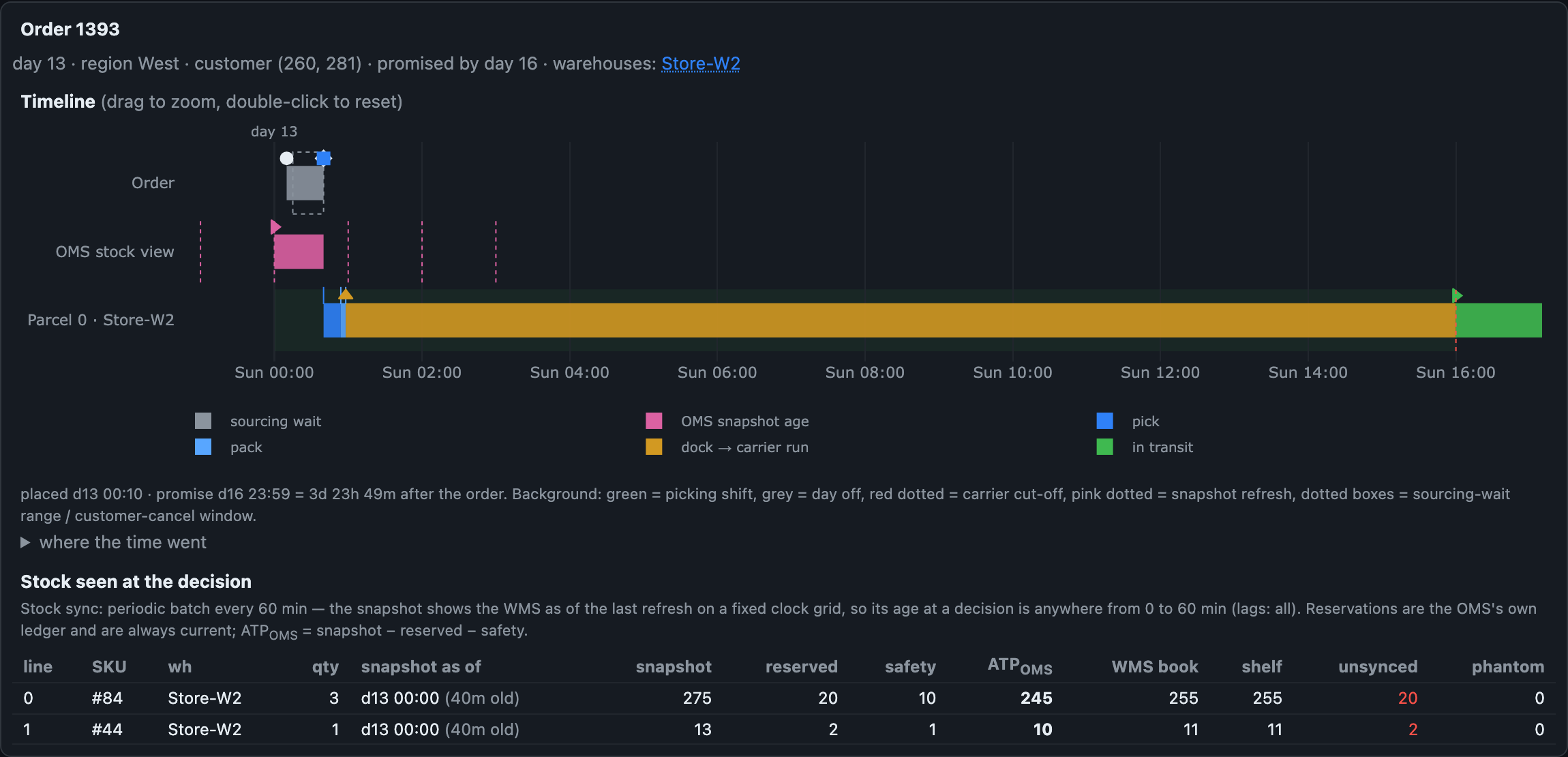
demo_omnichannel with an hourly stock export. In the "OMS stock view" lane, the pink segment is the snapshot's age at decision time, the pink dashed line is the update grid. In the table, the snapshot shows more than the WMS books (unsynced > 0): some units have already been picked for other orders, but the write-off hasn't reached the OMS yet. The same units sit in reserved, so the OMS's ATP isn't overstated.A note on holding goods in the cart. The engine has no separate "abandoned cart" entity, but its behavior can be reproduced through the order intake stage with early reservation enabled (reserve_during_checks: true, with p_hold: 0.3 as the share of abandoned carts and hold_hours_mean: 1.0 as the hold's TTL). This trick works great for visually checking the mechanics on the timeline, but for rigorous numerical measurements, keep in mind that in the current implementation, orders filtered out at intake inflate the network's calculated initial stock and end up in the denominator of per-order metrics.
Retail stores, in-store pickup (BOPIS), and returns
A warehouse in the simulator can be declared a retail store (tier: store). A store immediately gets different economics and a different way of life: low picking throughput (capacity_lines_per_day: 40), expensive manual labor by sales associates (handling_cost_per_line: 1.5), a modest courier truck limit, and, most importantly, a stream of walk-in shoppers (walkin_units_per_day: 60) who take goods right off the display from 9 a.m. to 9 p.m.
warehouses:
  - { warehouse_id: 2, name: Store-W1, tier: store, capacity_lines_per_day: 40,
      handling_cost_per_line: 1.5, walkin_units_per_day: 60,
      online_protect_units: 1, ship_online: true }
A shopper on the sales floor doesn't know that the last jacket on the rack was reserved for an online order ten minutes ago. They take it to the register and pay, and an hour later the online order picker records a walkin_conflict shortage. To keep the online storefront from sweeping the stores clean and pitting sales channels against each other, you set a protected display stock, online_protect_units: 1: the store hides the last unit of each product from the online channel for its walk-in customers.
Besides courier shipping from the store (Ship-from-Store), stores handle in-store pickup (BOPIS, Buy Online, Pick Up In Store; the share of such orders is set in bopis_share: 0.25). If all the goods are in the chosen store, the customer is promised pickup as early as tomorrow, and the company saves on delivery. If the store is short on some items, they're brought in from warehouses on a consolidated inter-warehouse run at 40% of the regular rate (ship_to_store_cost_factor: 0.4). On average, the shopper picks up the order 20 hours after it's ready, but 5% of customers never show up (p_no_show: 0.05): after five days of waiting, the box is broken down and put back on the shelf, with a penalty for the staff's wasted work.
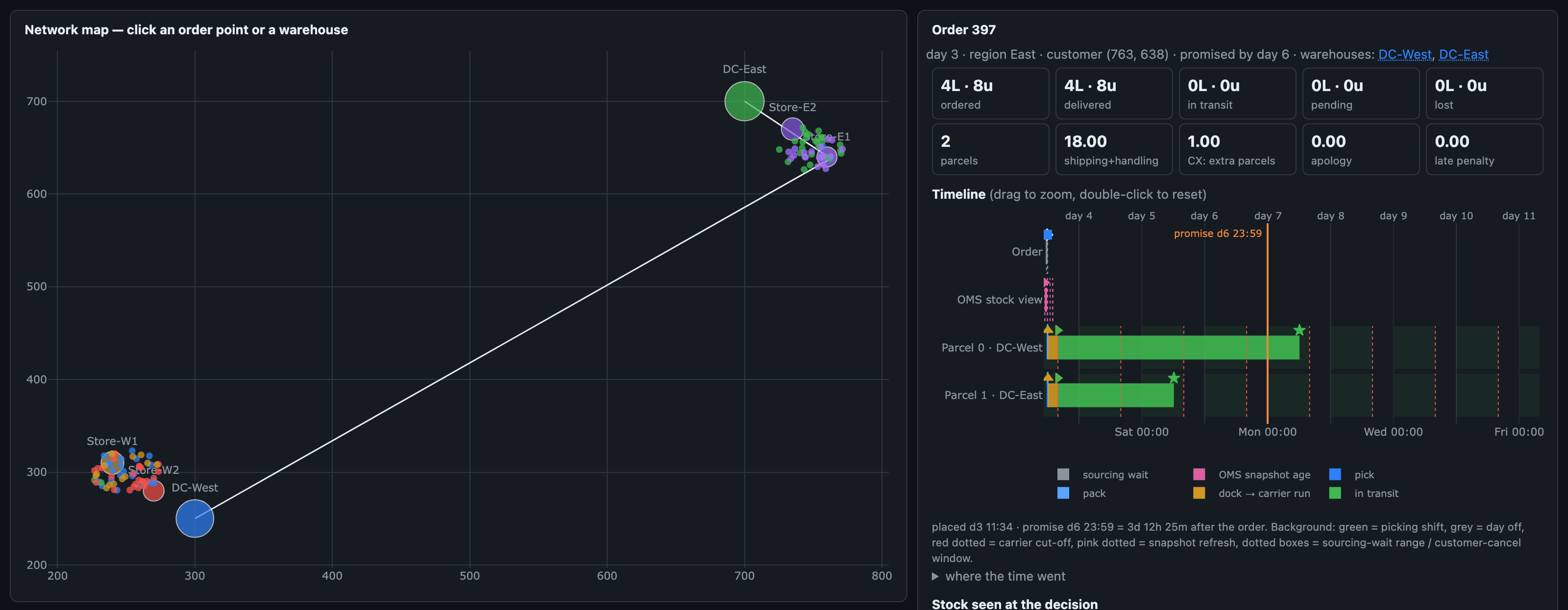
demo_omnichannel in the inspector: two DCs and four stores in two cities. The dots are one day's orders, colored by ship-from location. The selected order is split between two DCs: lines lead from the customer to both warehouses, and its card and timeline are on the right.Delivered orders may be partially returned after 3–14 days (returns.enabled: true). The return rate depends on the product category (clothing is returned 5 times more often than electronics) and jumps by split_uplift: 0.18 for each extra parcel the order was split into. Customers bring half of the returns to stores in person and mail the other half back at the store's expense. After inspection and repackaging (processing_cost_per_unit: 1.0), 80% of returned items go back into stock and become available for sale, and 20% are written off as defective.
Network balancing, Black Friday, and warehouse outages
At the network level, warehouses can exchange stock overnight (transfers.enabled: true): either a central hub (rdc) feeds the regional warehouses (fdc), or warehouses share surpluses directly when one has less than low_days: 5 days of stock left and a neighbor holds more than high_days: 15. To keep balancing algorithms from shuttling the same product back and forth in circles, there are built-in safeguards (cooldown_days, max_source_share) that keep the idle-transfer metric ping_pong_units at zero.
To test how the whole setup holds up in extreme conditions, the config has a shocks block (shocks):
shocks:
  enabled: true
  peak_multiplier: 4.0           # a fourfold demand spike ("Black Friday")
  peak_duration_days: 3
  peak_start_day: 20
  warehouse_outage_id: 0         # an outage and full shutdown of warehouse W0 for a week
  warehouse_outage_days: 7
  warehouse_outage_start_day: 14
During an outage, the warehouse disappears from the OMS's radar, and the whole flow of orders crashes down on its neighbors.
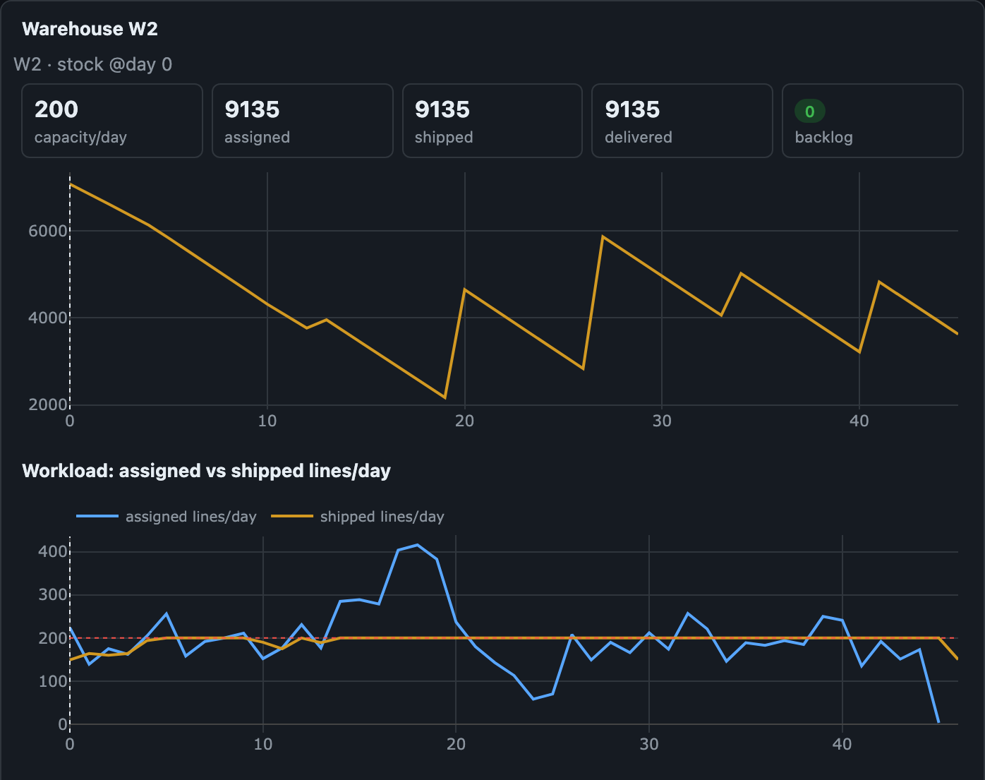
demo_showcase, with the network loaded almost to the limit. Warehouse W1 is closed on days 14–20. During the outage, neighbor W2 gets 280–420 lines a day against a capacity of 200, and its queue grows to almost a thousand lines. After W1 comes back, the queue melts slowly: there's almost no spare capacity to work it down.When the main simulation time sim_days ends, intake of new orders stops, and the system gets up to 60 days to "drain," finishing the picking and delivery of commitments already accepted. Anything stuck in queues that didn't arrive even within that time is written off as hopelessly failed and marked horizon, a sure sign that the network choked.
What the experiments on the testbed showed
Once this whole construction kit was assembled and equipped with the osbench sweep batch runner and the osbench tune weight optimizer, I ran a series of thirteen computational studies on it. Some of the results turned out to be quite instructive and at times contradicted the usual industry intuition. More on them separately.
If you're the rare reader who made it this far, I'd be glad if you shared hypotheses that could be tested on this testbed. You can reach me here: Rauf Aliev
Discussion
Powered by GitHub Discussions — sign in with a GitHub account to join the conversation.