SIHG4SR — Side Info Heterogeneous Graph for Session Recommender
Full annotated transcript (verbatim, reconstructed by speaker) · Intel team's RecSys Challenge 2022 solution talk (recording in progress)
Monday, October 5, 2026 · 13:37–13:46 · Intel (presenter) — recorded talk
Who's speaking
Chendi Xue — Presenter (Intel, US)Unidentified voice — opening fragment
How to read this — the callouts
🆕 NEWSomething we did not have in the source material before this session.
✅ CONFIRMSConfirms / adds colour to something already documented.
🔄 UPDATESChanges, narrows, or contradicts what prior sources said — worth reconciling.
This is the full transcript — every topic discussed is here, reconstructed into clean speaker turns from the verbatim recording (nothing dropped; only obvious speech-to-text garbles fixed). Skim the coloured callouts for takeaways; read the turns for detail. The session is still being recorded, so the transcript ends abruptly at 13:46:16, just after the "Workflow" slide (13:46:56) appeared.
1 · Opening and introduction of SIHG4SR
Unidentified voiceStart of recording13:37:43
…the video.
Chendi XueIntel · Presenter13:37:45
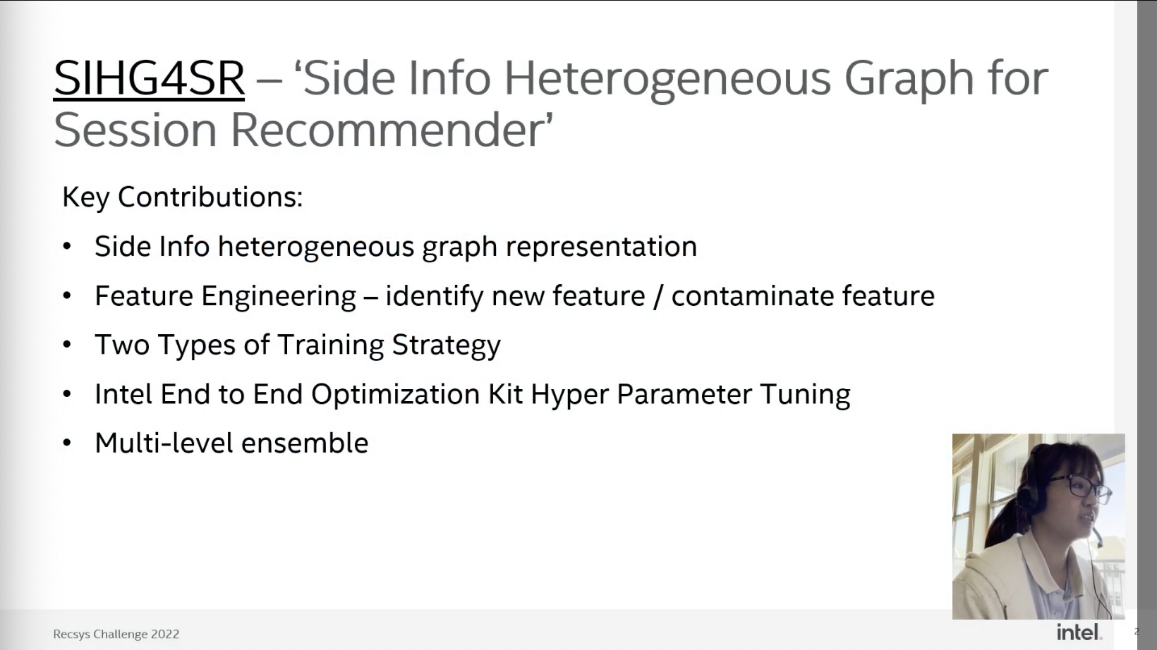
Okay, hi, this is Chendi Xue. I'm from Intel, and this is our team. We use SIHG4SR, which stands for Side Info Heterogeneous Graph for Session Recommender System Problem.
13:38:02Title slide — SIHG4SR – Side Info Heterogeneous Graph for Session Recommender. Authors: Chendi Xue (Intel, US), Xinyao Wang (Intel, China), Yu Zhou (Intel, China), Ke Ding (Intel, US), Jian Zhang (Intel, China), Rita Brugarolas Brufau (Intel), Eric Anderson (Intel, US). Confirms the presenter's name and corrects the method name heard as "Site Information".
2 · Key contributions of the solution
Chendi XueIntel · Presenter13:38:00
So since we only have 10 minutes, so I just include the key contributions from our solution in this slide. I will talk about the graph, the side info heterogeneous graph representation. Then there are four main contributions, which are feature engineering, the training strategy, the hyperparameter tuning, and the multi-level model ensemble.
13:38:10"Key Contributions" slide (RecSys Challenge 2022): side info heterogeneous graph representation; feature engineering — identify new feature / contaminate feature; two types of training strategy; Intel End to End Optimization Kit hyperparameter tuning; multi-level ensemble. Used to fix "speech engineering", "hyperparameterity" and "multilevel model example".
3 · Model architecture: heterogeneous graph, two channels, weighted loss
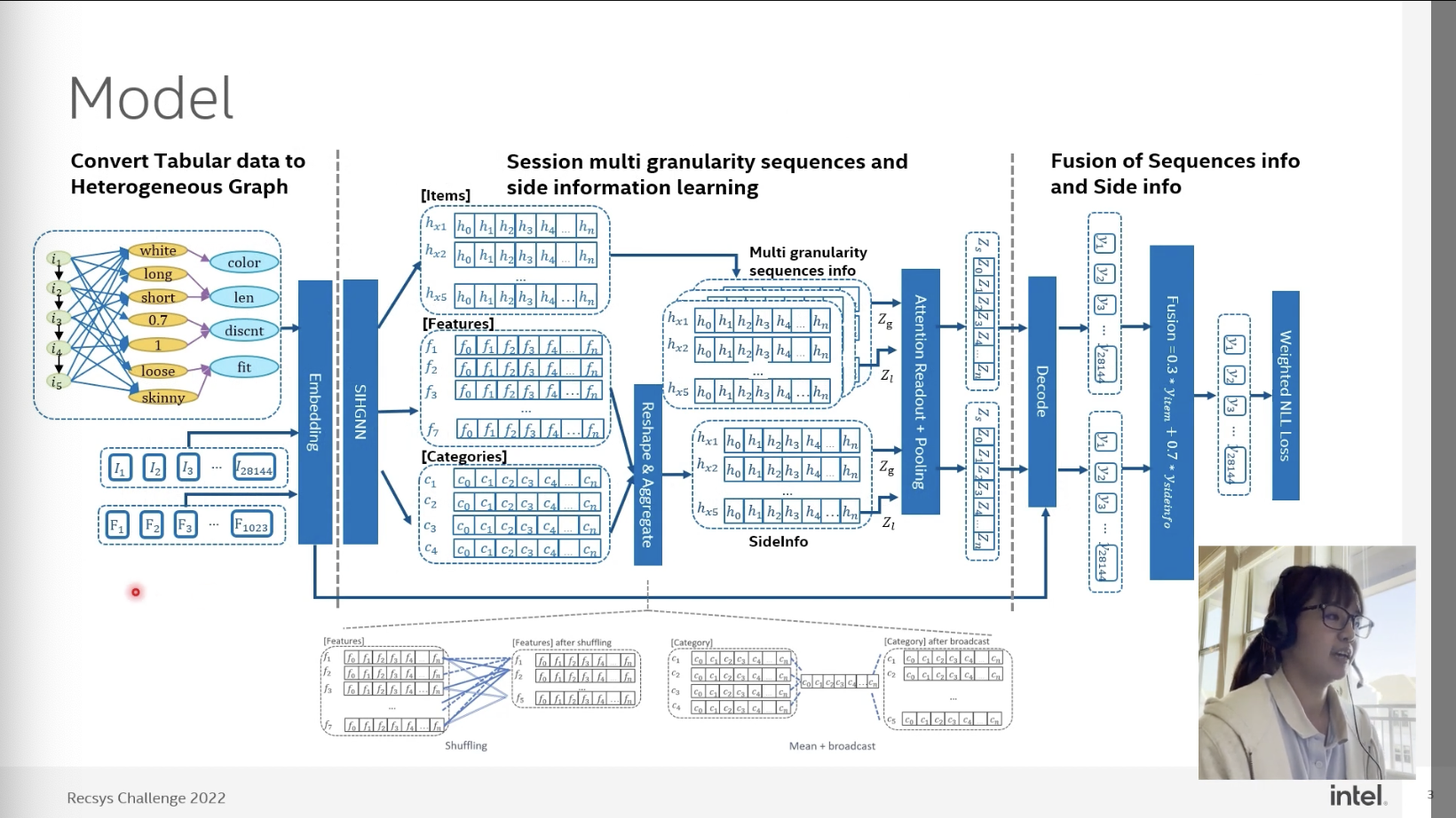
13:38:41"Model" slide, a three-stage pipeline: (1) convert tabular data to a heterogeneous graph (items linked to feature values such as color, length, discount and fit) → Embedding → SIHGNN; (2) session multi-granularity sequence and side information learning (items, features, categories → reshape & aggregate with shuffling and mean + broadcast → attention readout + pooling); (3) fusion of sequence info and side info (Fusion = 0.3·yitem + 0.7·ysideinfo) → weighted NLL loss over 28,144 candidate items. Chendi walks through this slide in the turn below; it is the source for "GNN", "tabular data" and "side".
Chendi XueIntel · Presenter13:38:31
Okay, so for the model, we are simply using a GNN-based model. So there are three phases in our model. The first phase is to convert the tabular data to the heterogeneous graph. I think you already know that there are multiple sessions in this dataset. Actually, there are one million sessions in this dataset. So each session will be built into a graph, like the one at the side.
And so there are three types of nodes in the graph. The first type of node is item, which means when the user views one item, then the next item, and the next item, it will just link as the item sequence. Then we are using a second type of node, which is a feature. Since the feature data in the dataset is anonymous, but we are trying to think of the features as meaning something. So we can think like the feature maybe means like the color is white, the length is long, the discount is 70%, something like that. Then we can think of like we are to link the item to the corresponding feature. Then there is a third type of node, which is category, which means what is the feature category of this feature. And then we do this heterogeneous graph.
Then we're feeding this heterogeneous graph into our GNN. And then we will have three types of embedding table because we have three types of nodes. Then the embedding tables are item, feature, and the category. So we didn't aggregate these three types of nodes immediately, but we use two channels to propagate these two types of information. The first channel… The first channel is only for the items, like this channel, and the second channel is for feature and the category aggregation. So it's very straightforward to think of why we use the first channel only for the item, because this is the main information. And then this is something about the side information, which is the feature and the category.
And to here, you can see there is a problem, because for the feature, the number of nodes is seven, but the item is only five. So how can I aggregate these two pieces of information together? This is how we are doing different types of reshape to the original embedding table. For feature, we will, we will try to do the shuffling, which means like where white belongs to item one, item two, and item five, we will just add feature one to item one, item two, and item five. Then we will, we will have a new reshaped embedding table, which shares the same size as the item. Then for the category, we try to just do a mean and the broadcast, because the category is more general information. Then we add these two reshaped embedding tables together and decode as the second logit.
Then we fuse these two channels of logits together to get our final logit, and use a weighted loss. Weighted loss here means — because this is a question about fashion, which means the most recent data will tell us more than the maybe one-year-ago data. So this is why we're using a weight to tell us that the data is recent or the data is years ago. So this is how we build our model. So we can predict the candidate items with the highest scores on the right side. [garbled in the recording: “that kind of document with a really great course”]
4 · Contribution 1: graph & feature engineering
Chendi XueIntel · Presenter13:42:27
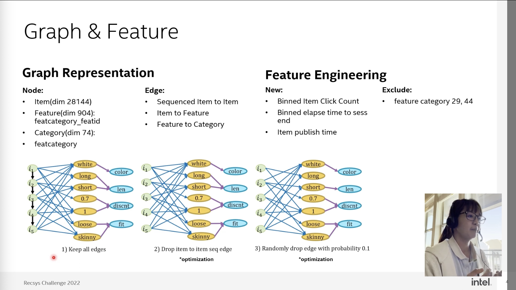
And then there are, as I mentioned, there are four key contributions to improve our score. The first one is the feature engineering work. So you already know that there are three types of nodes and three types of edges in our graph. Then we are thinking that putting which kind of node into the graph maybe will either contaminate or contribute to the final score. This is how we are trying to just exclude one category or feature each time, to see if there are some categories maybe just contributing some conflicting information into our GNN, which brought the score down. This is why we exclude the categories 29 and 44.
Then we also think about if there is any chance that we can build new features into the graph, which is because we have the timestamp in the dataset, and we are thinking this is a very good source for new features. So there are three new types of feature we are creating. One is we just do statistics on the history item click count, to say, oh okay, this item is hot, it was clicked multiple times, and this item was only clicked one or two times. And the second feature is the elapsed time to the session end. Why are we adding this type of information? Because you can think that if one user opened a session maybe two hours ago, then she or he does the purchase at the last one minute. So the items she or he viewed in the last five minutes contribute more to her or his decision than the item from two hours ago. This is why we are using the elapsed time as a new feature. Then the feature item publish time, this is another type of new feature.
13:43:12"Graph & Feature" slide. Nodes: Item (dim 28,144), Feature (dim 904, featcategory_featid), Category (dim 74, featcategory). Edges: sequenced item → item, item → feature, feature → category. New features: binned item click count, binned elapsed time to session end, item publish time. Excluded: feature categories 29 and 44. Bottom: 1) keep all edges, 2) drop item-to-item sequence edges, 3) randomly drop edges with probability 0.1 (both marked "*optimization"). Used to fix "statistics or the history item click count" and "item published time".
Chendi XueIntel · Presenter≈13:44
So besides the new features we are creating, we are also thinking about whether there is any chance we should drop the edges. This is what we draw in the bottom part of this slide. So firstly we keep all the edges, which are the item sequence edges, the item-to-feature edges, and the feature-to-category edges. Then we try to just remove the item sequence edges, because we already have the elapsed time, so we don't need to use the sequence. Then we also try to do a random drop of the edges with a probability of 0.1, which helps us to fix the overfitting issue.
5 · Contribution 2: training strategy (next-click pre-training)
Chendi XueIntel · Presenter≈13:45
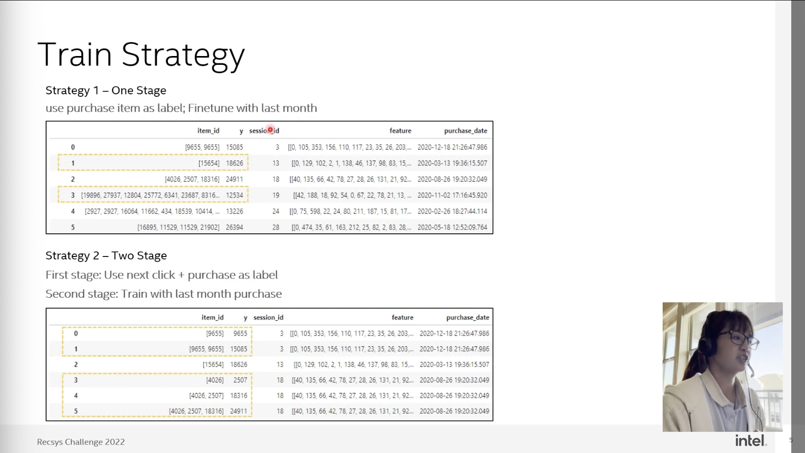
Okay, then the second key contribution is the training strategy. So we are using two types of training strategies. The first one is just to load in the dataset, create a graph for each record, and then train using the purchase item as a label. Then we're thinking that since the next click also reveals the user's intention, right, so how about we use the next click to pre-train the model, then we use the real purchase item to train the model. It's something like borrowing from transfer learning: we can train a model with a bigger dataset, and then we train on the real problem.
13:45:34"Train Strategy" slide. Strategy 1, one stage: use the purchase item as label, then fine-tune on the last month. Strategy 2, two stage: first stage uses next click + purchase as labels, second stage trains on last-month purchases. Sample tables show how session 3 ([9655, 9655] → 15085) and session 18 ([4026, 2507, 18316] → 24911) are expanded into prefix → next-click rows. Used to fix "train strategy" and "reviews the user's intention".
Chendi XueIntel · Presenter13:46:16
So what we do here is: the first session is something like this. Then we augment it into two sessions. The first one is the first click, with the next click as its label. Then the second one is the whole session with the purchase item. And then, because the dataset is too big, we found that only using the last six months of the dataset is already enough. And this is how we use the training strategy to improve the score.
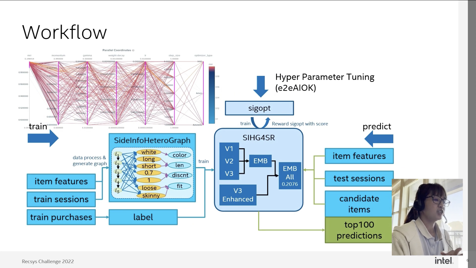
13:46:56"Workflow" slide. Train: item features + train sessions → data processing & graph generation → SideInfoHeteroGraph; train purchases → label. SIHG4SR variants V1, V2, V3 are combined (EMB), then ensembled with V3 Enhanced into EMB All = 0.2076. Hyperparameter tuning (e2eAIOK) uses SigOpt, which is rewarded with the score; the parallel-coordinates plot shows MRR against momentum, gamma, weight decay, lr, step size and optimizer type. Predict: item features + test sessions + candidate items → top-100 predictions. The recording snapshot ends before this slide is explained aloud.